Research article

Assessing future drought evolution and driving mechanisms in the Weigan River Basin under CMIP6 climate scenarios

  • WANG Wenbo 1, 2 ,
  • LIN Li , 1, 2, * ,
  • CHEN Dandan 1, 2 ,
  • YANG Jiayun 1, 2
Expand
  • 1 College of Hydraulic and Civil Engineering, Xinjiang Agricultural University, Urumqi 830052, China
  • 2 Xinjiang Key Laboratory of Hydraulic Engineering Security and Water Disasters Prevention, Urumqi 830052, China
*LIN Li (E-mail: )

Received date: 2025-07-30

  Revised date: 2026-01-08

  Accepted date: 2026-01-30

  Online published: 2026-03-12

Abstract

In the northern Tarim River Basin, the Weigan River Basin is a critical endorheic system characterized by extreme aridity, where drought poses a major natural hazard to agricultural production and ecological stability. This study assessed the future evolution of drought under climate change by employing the standardized moisture anomaly index (SZI) on the basis of multi-model the Coupled Model Intercomparison Project Phase 6 (CMIP6) simulations under historical conditions (1970-2014) and future scenarios (shared socioeconomic pathway (SSP)1-2.6, SSP2-4.5, SSP3-7.0 and SSP5-8.5 for 2015-2100). The results show that precipitation-evapotranspiration anomalies are projected to first decline but then increase over time, with increased fluctuations and uncertainty under high-emission scenarios (SSP5-8.5). These trends indicate intensifying drought risks and reveal a strong influence of emission pathways on regional water cycling. Temporal analysis of SZI indicates a transition from wetting to drying under low- and medium-emission pathways (SSP1-2.6 and SSP2-4.5), whereas high-emission scenarios are characterized by persistent drying and increased variability. The significant lower-tail dependence (0.271) observed under SSP2-4.5 and SSP5-8.5 suggests that extreme droughts may be subject to nonlinear co-amplification across scenarios. The frequency of moderate and more severe drought events is expected to increase substantially, especially under SSP5-8.5, where drought occurrence is predicted to extend into spring and autumn and become more evenly distributed throughout the year. Spatially, drought duration shows significant positive autocorrelation across all scenarios, with hot spots consistently concentrated in the southern and southeastern regions of the basin. Random forest analysis, interpreted as association-based pattern attribution, indicates that meteorological variables (precipitation and potential evapotranspiration (PET)) make the greatest contributions to the hot spot pattern, followed by topography and soil moisture. Among land use categories, farmland generally shows higher drought sensitivity than other land use types, as reflected by its relative contribution patterns across scenarios. The spatial pattern of drought is statistically structured by climatic forcing, surface conditions, and soil moisture status, reflecting their coupled associations with hot spot occurrence. In addition, a drought spatial uncertainty index was constructed from multi-scenario hot spot maps, revealing spatially heterogeneous structural variability throughout the basin. Correlation analysis further highlights strong internal couplings among environmental variables (e.g., elevation-linked hydroclimatic gradients and grassland-bare soil contrasts). These findings offer a scientific basis for developing region-specific drought monitoring and adaptation strategies under future climate change conditions.

Cite this article

WANG Wenbo , LIN Li , CHEN Dandan , YANG Jiayun . Assessing future drought evolution and driving mechanisms in the Weigan River Basin under CMIP6 climate scenarios[J]. Journal of Arid Land, 2026 , 18(2) : 235 -262 . DOI: 10.1016/j.jaridl.2026.02.003

1 Introduction

Escalating global temperatures have intensified the hydrological cycle, leading to increased frequency and severity of regional drought events (Li et al., 2024). This trend is particularly evident in the mid-latitudes of the Northern Hemisphere, where the accelerated global hydrological cycle driven by climate change has significantly increased the frequency of droughts and other extreme hydrological events (Li et al., 2023b). The combined effects of population growth and the expansion of agricultural and industrial activities have further exacerbated water scarcity. This issue is particularly severe in arid areas (Liu et al., 2017). Moreover, drought disasters inflict substantial losses on ecosystems, socioeconomic systems, and agricultural production (Orimoloye et al., 2021), posing a persistent threat to food and ecological security. Statistics show that drought accounts for approximately 35.00% of the total economic losses caused by natural disasters (Hanby et al., 2025). Therefore, investigating the spatiotemporal variations and evolutionary patterns of drought is crucial for enhancing societal resilience and promoting stable economic development.
The Tarim River Basin is a critical economic zone and an ecologically sensitive and fragile area in Xinjiang Uygur Autonomous Region, China. It covers a vast area, including nine major source rivers and 144 river systems in total (Li et al., 2023a). Notably, climatic characteristics and their temporal variations differ markedly across its subregions. Owing to its inland location deep within the Eurasian continent and its remoteness from the oceans, drought events frequently occur (Yang et al., 2019). Since 2000, approximately 65.00% of the northern margin of the Tarim River Basin has experienced intensified drought, with an overall trend indicating continued aridification in the future (Ding et al., 2024). The increasing severity of drought in the Tarim River Basin has drawn widespread attention. Using historical meteorological data and global climate models (GCMs), Wang (2022) examined the drought characteristics in the basin and reported that from 1970 to 2019, the annual mean temperature increased significantly at a rate of 0.411°C/10a. Moreover, the standardized precipitation evapotranspiration index (SPEI) exhibited an overall increasing trend, suggesting that future increases in temperature and potential evapotranspiration (PET) are ongoing. Xiang et al. (2024) used the Coupled Model Intercomparison Project Phase 6 (CMIP6) climate model outputs and the Hydrologic Engineering Center's-Hydrologic Modelling System (HEC-HMS) hydrological model, together with historical data, to show that future hydrological droughts in the Yarkant River Basin will substantially exceed historical levels in terms of duration, intensity, severity, and peak magnitude, with droughts becoming more frequent and severe. Guo et al. (2017) systematically analyzed drought conditions in the Tarim River Basin using remote sensing data and the modified perpendicular drought index (MPDI), and further applied rescaled range (R/S) analysis to investigate the persistence of drought dynamics. Their results revealed persistent and widespread drought conditions in certain upstream and midstream areas of the basin. By analyzing changes in the water cycle and water balance in the Aksu River Basin, Li (2015) evaluated drought evolution and revealed that drought progression is characterized by complex characteristics and has intensified in both oasis and desert areas. Ding et al. (2024) applied a Bayesian network model to estimate the conditional probability between meteorological and hydrological droughts and examined the likelihood of hydrological drought under different scenarios in the Tarim River Basin. The results indicated that future climate change will alter the frequency and intensity of both meteorological and hydrological droughts. Overall, significant progress has been made in the study of drought-related issues in the Tarim River Basin and its subregions. However, most existing studies have relied on traditional methodologies and conventional drought indices, often yielding only descriptive findings and lacking in-depth analysis of underlying mechanisms.
The Weigan River is one of the nine major tributaries of the Tarim River, and its riparian zones constitute a vital agricultural and ecological oasis. Amid increasing water demand and the impacts of climate change, the Weigan River Oasis is facing challenges such as water shortages, ecological degradation, and land desertification (Wang et al., 2013). Therefore, rational water resource management and sustainable development strategies are becoming increasingly critical. Although limited research has focused specifically on drought in the Weigan River Basin, comprehensive analyses of future spatiotemporal drought trends remain insufficient. A comprehensive multi-scenario assessment of future drought in the Weigan River Basin—particularly one that examines nonlinear dependencies in extreme events and spatial uncertainties using CMIP6 models—remains lacking.
The CMIP6 was officially approved for planning in autumn 2012 by the Working Group on Coupled Modelling (WGCM) under the World Climate Research Programme (WCRP), with model development and experimental design completed in 2017 (Eyring et al., 2016; Zhou et al., 2019). Compared with its predecessor, Coupled Model Intercomparison Project Phase 5 (CMIP5), CMIP6 has made substantial advancements in simulating physical climate processes and has reduced uncertainties in the simulation of precipitation, temperature, and other variables. By incorporating shared socioeconomic pathways (SSPs) alongside radiative forcing targets, CMIP6 has enhanced the socioeconomic dimension of future climate projections. Its multi-model ensemble (MME) outputs have provided a critical scientific foundation for the Intergovernmental Panel on Climate Change (IPCC) Sixth Assessment Report, specifically for regional precipitation changes and extreme event risk assessments. These developments have provided a rich dataset that supports global climate research and laid a solid foundation for assessing the impacts and risks of climate change on energy, water resources, and agriculture (Zhang et al., 2021a; Tian et al., 2023; Liu et al., 2024). CMIP6 simulation results are expected to serve as a key reference for future climate change research. The CMIP6 historical baseline period spans 1850-2014 and is used to validate model performance, with all scenario simulations beginning in January 2015, immediately after the historical simulation period ended in December 2014.
Despite the increasing application of CMIP6 projections in drought assessments, existing studies in arid inland basins have rarely integrated physically based drought indices with event-scale characteristics and spatial clustering analyses to systematically examine the long-term evolution of drought under climate change. In this study, CMIP6 multi-model climate projections were employed to derive the standardized moisture anomaly index (SZI) for the Weigan River Basin under historical (1970-2014) and future (2015-2100) climate conditions. By applying run theory, Bayesian piecewise linear regression, and spatial autocorrelation analysis, this study aims to characterize the duration and frequency of drought events, identify their spatial clustering patterns, and quantify the future spatiotemporal evolution of drought events under different emission pathways in the Weigan River Basin. The results provide a physically informed and spatially explicit perspective on drought dynamics in an arid basin, thereby improving the understanding of how drought characteristics may evolve under climate change and offering a scientific basis for drought risk assessment and adaptive water resources management in similar arid areas.

2 Materials and methods

2.1 Study area

The Weigan River originates from the continental glacier region of Khan Tengri Peak, which is located on the southern slope of the Tianshan Mountains. The river is formed by the confluence of tributaries, including the Muzart River and the Kizil River, and extends approximately 452 km, with a drainage area of approximately 72,400.00 km2 (Fig. 1). The river flows through Baicheng, Kuqa, Xinhe, and Xayar counties within Aksu Prefecture. The Weigan River Basin (40°57′00″-42°23′24″N, 80°37′48″-83°31′12″E) features a typical continental warm-temperate and extremely arid climate, with long-term mean annual temperatures ranging from 10.500°C to 11.400°C and an average annual precipitation ranging from 50.500 to 66.500 mm. The mean annual evaporation is extremely high, ranging from 2000.700 to 2092.000 mm (Ke et al., 2020). Precipitation shows significant spatial and temporal variability, primarily occurring between June and September each year. Due to excessive irrigation withdrawals along its course, compounded by the effects of climate change, the Weigan River no longer discharges into the Tarim River.
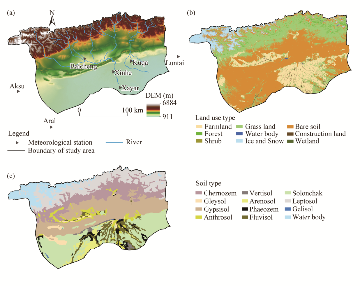
Fig. 1 Regional overview of the digital elevation model (DEM) (a) and distribution of land use types (b) and soil types (c) in the Weigan River Basin

2.2 Data source

In this study, monthly outputs from seven CMIP6 GCMs were used, including precipitation, minimum, maximum, and mean temperature, solar radiation, wind speed, and relative humidity for the historical baseline (1970-2014) and the future projection period (2015-2100). Four SSPs (SSP1-2.6, SSP2-4.5, SSP3-7.0, and SSP5-8.5) were analyzed. Model selection was on the basis of the data completeness required for the Penman-Monteith PET calculation, which depends on six key variables (minimum, maximum, and mean temperature; relative humidity; wind speed; and solar radiation). After systematic screening, only seven models provided the complete variable set across the historical experiment and the future SSP experiments (Table 1).
Table 1 Basic information on the seven global climate models (GCMs) of the Coupled Model Intercomparison Project Phase 6 (CMIP6)
GCMs Country Institute Spatial resolution
CanESM5-1 Canada Canadian Centre for Climate Modelling and Analysis (CCCma) 2.800°×2.800°
FGOALS-g3 China Chinese Academy of Sciences (CAS) 2.000°×2.000°
INM-CM4-8 Russia Institute of Numerical Mathematics, Russian Academy of Sciences (INMRAS) 1.875°×1.241°
INM-CM5-0
MIROC6 Japan Japan Agency for Marine-Earth Science and Technology (JAMSTEC) 1.400°×1.400°
MRI-ESM2-0 Meteorological Research Institute (MRI) 1.125°×1.125°
MPI-ESM1-2-LR Germany Max Planck Institute for Meteorology (MPI-M) 1.875°×1.875°
Using a limited but complete ensemble is consistent with recent drought and climate studies, in which data availability and representativeness are prioritized over ensemble size (Zhai et al., 2020; Behzadi et al., 2024; Soares et al., 2024). Small-to-medium ensembles (5-10 models) have been shown to capture the main uncertainty range effectively (Pathak et al., 2023). Moreover, these seven models originate from distinct international modeling centers, providing structural diversity and broad representativeness.
Observational data were obtained from the China Meteorological Data Service Center (http://data.cma.gov.cn/), comprising daily meteorological records (precipitation; minimum, maximum, and mean temperature; relative humidity; wind speed; and sunshine duration) from 1970 to 2021 from seven stations located within and around the Weigan River Basin (Fig. 1a; Table 2). The normalized difference vegetation index (NDVI) was derived from the Moderate-resolution Imaging Spectroradiometer (MODIS) NDVI product (Terra), which was accessed via the National Aeronautics and Space Administration (NASA) Earthdata platform (https://earthdata.nasa.gov/). Land use data were derived from the China Land Cover Dataset (CLCD), developed by Wuhan University, China, which provides annual 30 m land cover maps for 1985-2023 (Fig. 1b). Soil data (soil type) were obtained from the Harmonized World Soil Database (HWSD) and accessed via the National Cryosphere Desert Data Center (http://www.ncdc.ac.cn) (Fig. 1c). The digital elevation model (DEM) was obtained from the Geospatial Data Cloud (https://www.gscloud.cn/), and slope was derived from the DEM. Soil moisture was derived from the SZI calculations, and its long-term mean was used in subsequent analyses.
Table 2 Geographic information of meteorological stations
Station Latitude Longitude Elevation (m)
Kuqa 41°43′12″N 83°04′12″E 1082
Luntai 41°46′48″N 84°15′00″E 977
Baicheng 41°46′48″N 81°54′00″E 1230
Aksu 41°10′12″N 80°13′48″E 1105
Aral 40°30′00″N 81°03′00″E 1013
Xinhe 41°31′48″N 82°37′12″E 1014
Xayar 41°13′48″N 82°46′48″E 981

2.3 Methods

2.3.1 Downscaling and bias correction

We applied a calendar-month delta-scaling approach to harmonize the CMIP6 outputs (approximately 1.000°-2.800°) with station-based observations. Both datasets were bilinearly interpolated to a common 0.250° grid for grid matching rather than to create new spatial detail. Bias correction was implemented in a grid-wise manner using calendar-month climatological factors derived over the historical overlap period (1970-2014). Precipitation was adjusted multiplicatively using the ratio of observed to simulated monthly climatologies, whereas temperature was adjusted additively using monthly mean offsets. This workflow preserves large-scale spatial gradients while reducing systematic mean-seasonal biases, and it is widely adopted in regional climate impact assessments (Lei et al., 2023; Soares et al., 2024).

2.3.2 Model evaluation method

To quantitatively evaluate the consistency between the downscaled simulations and observations, we employed three commonly used statistical indicators: percent bias (PBIAS), root mean square error (RMSE), and Nash-Sutcliffe efficiency (NSE). The PBIAS measures the relative magnitude and direction of the systematic deviation between simulated and observed values, the RMSE reflects the average magnitude of error, and the NSE indicates how well the simulated time series reproduces the observed variability. Together, these metrics provide a comprehensive assessment of model bias, accuracy, and reliability across variables. These metrics were computed at the daily scale by comparing bias-corrected model simulations with station observations for each variable, after spatially matching model grid values to station locations. The evaluation was conducted for both individual GCMs and the mean MME, enabling a consistent assessment of model skill and the benefits of ensemble averaging.
Taylor diagrams are widely used diagnostic tools for evaluating the performance of multiple climate models in relation to observational data. These diagrams integrate three key statistical metrics—the standard deviation (SD), correlation coefficient, and centered root mean square error (CRMSE)—to quantify the similarity between model simulations and observations. By presenting these metrics in a single polar coordinate plot, the Taylor diagram offers a concise and comprehensive visualization of model performance.
The SD reflects the degree of dispersion in the model data:
$\sigma =\sqrt{\frac{1}{n}{\displaystyle \sum _{i=1}^{n}{\left({x}_{i}-\overline{x}\right)}^{2}}}$
where σ is the SD; xi is the observed value of sample i; $\overline{x}$ is the mean of the observed data; and n is the sample size.
The correlation coefficient measures the linear relationship between the model predictions and observations:
$R=\frac{{\displaystyle {\sum }_{i=1}^{n}\left({x}_{i}-\overline{x}\right)\left({y}_{i}-\overline{y}\right)}}{\sqrt{{\displaystyle {\sum }_{i=1}^{n}{\left({x}_{i}-\overline{x}\right)}^{2}}}\sqrt{{\displaystyle {\sum }_{i=1}^{n}{\left({y}_{i}-\overline{y}\right)}^{2}}}}$
where R is the correlation coefficient; yi is the simulated value of sample i; and $\overline{y}$ is the mean of the simulated values. The value of R ranges from -1 to 1, with values closer to 1 indicating a stronger correlation.
The CRMSE evaluates the magnitude of the error between the model predictions and observations:
$\text{CRMSE}=\sqrt{\frac{1}{n}{{\displaystyle \sum _{i=1}^{n}\left[\left({y}_{i}-\overline{y}\right)-\left({x}_{i}-\overline{x}\right)\right]}}^{2}}$

2.3.3 SZI index

The SZI proposed by Zhang et al. (2015), is a standardized drought metric formulated within a water-energy balance framework to characterize moisture anomalies driven jointly by precipitation supply and atmospheric evaporative demand. The SZI integrates the physically based water-balance logic of the Palmer drought severity index (PDSI) with the multi-scalar standardization concept of the SPEI. The SZI leverages the variable infiltration capacity (VIC) model to represent key hydrological processes and derives standardized anomalies by estimating climatically appropriate precipitation and normalizing the resulting moisture departures. In this study, the SZI was adopted as a physically informed and comparable indicator to assess drought evolution across seasons and scenarios in an arid basin, without implying universal superiority over other indices. To facilitate the interpretation of drought severity, researchers usually classifies SZI values into five drought categories (Table 3). This approach has been shown to capture the onset, persistence, and termination of multiyear drought events and to mitigate the tendency of the SPEI to overamplify drought severity via PET in arid and semiarid environments (Zhang et al., 2021b).
Table 3 Drought classification using the standardized moisture anomaly index (SZI)
Drought level SZI
No drought SZI> -0.5
Light drought -1.0<SZI≤ -0.5
Moderate drought -1.5<SZI≤ -1.0
Severe drought -2.0<SZI≤ -1.5
Extreme drought SZI≤ -2.0
Calculating the PET is a key step in computing the SZI. In this study, monthly PET was estimated using the Penman-Monteith equation:
$\text{PET}=\frac{\Delta \left({R}_{n}-G\right)+\gamma \frac{900}{T+273}{U}_{2}\left({e}_{s}-{e}_{a}\right)}{\Delta +\gamma \left(1+0.34{U}_{2}\right)}$
where is the slope of the saturation vapor pressure curve (kPa/°C); Rn is the net radiation (MJ/m2); G is the soil heat flux (MJ/m2); γ is the psychrometric constant (kPa/°C); T is the air temperature (°C); U2 is the wind speed at a height of 2 m (m/s); es is the saturation vapor pressure (kPa); and ea is the actual vapor pressure (kPa).
Moisture anomaly:
$d=\mathrm{Pr}\text{e}-\widehat{P}=\mathrm{Pr}\text{e}-{\alpha }_{j}\text{PET}+{\beta }_{j}\text{PR}+{\gamma }_{j}\text{PRO}+{\delta }_{j}\text{PL}$
where d is the hydrological anomaly (mm); Pre is the actual precipitation (mm); $\widehat{P}$ is the climatically appropriate precipitation (mm); PET is the potential evapotranspiration (mm); PR is potential recharge (mm); PRO is potential runoff (mm); PL is potential loss (mm); and αj, βj, γj, and δj (j=1, 2,..., 12) are the weight factors for potential variables PET, PR, PRO, and PL, respectively. PR, PRO, and PL are derived from the soil moisture balance model, which simulates soil moisture dynamics using a two-layer bucket model. We determined the weighting factors αj, βj, γj, and δj for each potential variable from the ratio of long-term mean observed hydrological elements to their potential values during the study period, and we further adjusted them to reflect the study area's monthly climatic conditions.
A three-parameter log-logistic distribution, which is consistent with the method used in the SPEI, is fitted to the probability distributions of water surplus and deficit:
$f\left(x\right)=\frac{\left(\frac{\alpha }{\beta }\right){\left(\frac{x-\theta }{\beta }\right)}^{\alpha -1}}{{\left[1+{\left(\frac{x-\theta }{\beta }\right)}^{\alpha }\right]}^{2}}$
where x denotes the accumulated water surplus or deficit (mm); and α, β, and θ are the shape, scale, and location parameters of the water surplus or deficit distribution, respectively.
The cumulative distribution function (CDF) is calculated as follows:
$F\left(x\right)=\frac{1}{1+{\left(\frac{x-\theta }{\beta }\right)}^{-\alpha }}$
The SZI time series is derived by applying a standard normal transformation:
$\text{SZI}={\varphi }^{-1}\left[F\left(x\right)\right]$
where ϕ-1 denotes the inverse standard normal distribution.

2.3.4 NDVI-SZI anomaly and lag analysis

Basin-mean monthly SZI and MODIS NDVI over 1985-2014 were transformed into calendar-month standardized anomalies (z anomalies) by removing the mean seasonal cycle separately for each calendar month (i.e., subtracting the long-term calendar-month mean and normalizing by the corresponding calendar-month SD). This transformation places both series on a dimensionless and seasonality-removed scale and facilitates comparability across months.
The NDVI-SZI association was quantified using Pearson correlation (linear dependence) and Spearman's rank correlation (monotonic dependence). In addition to linear regression, locally estimated scatterplot smoothing (LOESS) was applied as a nonparametric method to visualize the underlying trend in the NDVI-SZI relationship without imposing a predefined functional form. Spearman's coefficient was computed as:
$\rho =corr\left(rank\left(x\right),rank\left(y\right)\right)$
where 𝜌 is the Spearman rank correlation coefficient; and 𝑥 and 𝑦 denote paired SZI and NDVI z anomalies, respectively.
To evaluate delayed vegetation response, we conducted a lag analysis by correlating NDVI at time t with antecedent SZI at time (t lag) for candidate lags of 0-6 months (a positive lag indicates NDVI responding after SZI). After aligning the shifted series and removing missing pairs, we assessed statistical significance using autocorrelation-adjusted P values computed with an effective sample size correction:
${N}_{\text{eff}}=m\frac{1-{r}_{1x}{r}_{1y}}{1+{r}_{1x}{r}_{1y}}$
where Neff is the effective sample size accounting for serial autocorrelation; m is the number of paired samples for a given lag; and r1x and r1y are the lag-1 autocorrelations of the aligned SZI and NDVI anomaly series, respectively. Multiple testing across lags was controlled using the Benjamini-Hochberg false discovery rate (BH-FDR) applied to P, yielding qFDR; significance was evaluated at α=0.05.

2.3.5 Bayesian piecewise linear regression model

In this study, a Bayesian piecewise linear regression framework was applied to examine long-term trends in the SZI, with breakpoint locations and segment-specific slopes jointly estimated from posterior distributions and their associated uncertainties characterized using Bayesian credible intervals. A trend was considered statistically significant when the credible interval of the slope did not include zero (Brilleman et al. 2017).
Piecewise linear mode:
$y=\left\{{}_{{\Phi }_{0}+{\Phi }_{1}t+{\Phi }_{2}\left(t-c\right)+\epsilon \left(t\ge c\right)}^{{\Phi }_{0}+{\Phi }_{1}t+\epsilon \begin{array}{cc}& \end{array}\begin{array}{cc}& \end{array}\left(t<c\right)}\right.$
and Bayesian inference:
$p\left({\Phi }_{0},{\Phi }_{1},{\Phi }_{2},c,{\sigma }_{\epsilon }\left|y\right.\right)\propto p\left(y\left|\Phi,\right.c,{\sigma }_{\epsilon }\right)\times p\left(\Phi \right)\times p\left(c\right)\times p\left({\sigma }_{\epsilon }\right)$
where y is the response variable (i.e., SZI in this study); t is the independent variable representing time (a); Ф0 is the global intercept; Ф1 is the slope of the first segment; Ф2 is the incremental slope of the second segment relative to the first; c represents the breakpoint location; ε~N(0, σ2) is the Gaussian error term; and 𝜎𝜀 is the SD of the model residuals.

2.3.6 Vine copula model

Copula functions allow the marginal distributions of variables to be modeled independently from their dependence structures, making them suitable for describing nonlinear and asymmetric dependence. In this study, a pair-copula (vine) construction was adopted to flexibly characterize the dependence between SZI and related variables by decomposing the multivariate joint distribution into a sequence of bivariate copulas. This framework allows different copula families to be selected for different variable pairs, enabling the representation of asymmetric tail dependence that is relevant for drought analysis (Wu et al. 2021). The Akaike information criterion (AIC), which balances model goodness of fit against model complexity, was used to select the optimal copula family among competing candidates.
Bivariate vine copula joint density:
$f\left(u,v\right)=a\left(u,v\right)\times {f}_{1}\left(u\right)\times {f}_{2}\left(v\right)$
where a is the bivariate copula density; f1 and f2 are the marginal densities; and u and v denote the probability-integral-transformed marginal variables on [0,1].
Empirical cumulative distribution function (ECDF):
$\widehat{{F}_{m}}\left(x\right)=\frac{1}{m}{\displaystyle \sum _{i=1}^{m}{I}_{{x}_{i}}\le x}$
where I is the indicator function.
Tail dependence characterizes the strength of dependence between two variables in their joint extremes. For a bivariate copula with uniformly distributed marginal variables u and v on the interval [0,1], the lower-tail dependence coefficient λL measures the probability of joint extreme low values, while the upper-tail dependence coefficient λU quantifies the probability of joint extreme high values.
${\lambda }_{L}=\underset{q\to {0}^{+}}{\mathrm{lim}}P\text{'}\left(u\le q\left|v\le q\right.\right)$
${\lambda }_{U}=\underset{q\to {0}^{-}}{\mathrm{lim}}P\text{'}\left(u>q\left|v>q\right.\right)$
$\left\{\begin{array}{l}\widehat{{\lambda }_{L}}=\frac{1}{q}\times \frac{1}{m}{\displaystyle \sum _{i=1}^{m}{I}_{{u}_{i}\le q,\begin{array}{cc}& \end{array}\left({v}_{i}\le q\right)}}\\ \widehat{{\lambda }_{U}}=\frac{1}{q}\times \frac{1}{m}{\displaystyle \sum _{i=1}^{m}{I}_{{u}_{i}>1-q,\left({v}_{i}>1-q\right)}}\end{array}\right.$
where $\widehat{{\lambda }_{L}}$ and $\widehat{{\lambda }_{U}}$ are the empirical estimators of the lower- and upper-tail dependence coefficients, respectively, computed from finite samples; P' denotes the probability; q is the quantile threshold, and in this study, q=0.05; and ui and vi denote the ith paired observations of the transformed variables u and v, respectively, obtained by applying the empirical cumulative distribution functions to the original data.

2.3.7 Run theory

Run theory is a widely used time series analysis method in drought research and is commonly employed to identify and characterize drought events. By defining a drought threshold, the time series is divided into positive and negative runs, where positive runs represent periods when the index exceeds the threshold and negative runs correspond to periods when it remains below the threshold. A continuous negative run below the drought threshold is identified as a drought event.
Drought duration is defined as the number of consecutive time steps during which the SZI remains below the drought threshold, while drought frequency is defined as the ratio of the number of drought events (i.e., episodes with SZI≤threshold) to the total number of months in the study period. In this study, moderate or more severe drought events were identified using a standardized threshold of SZI≤ -1.0. Because the SZI represents standardized anomalies relative to local climatology, this threshold remains applicable in extremely arid basins where absolute precipitation amounts are small (Wang et al., 2022). The mean drought duration and frequency were used to quantify changes in drought characteristics in the Weigan River Basin under future climate scenarios.

2.3.8 SZI regression attribution

To characterize the relative influence of hydroclimatic water supply and atmospheric evaporative demand on historical SZI variability, we related basin-mean monthly SZI to precipitation and PET using a multiple linear regression over 1970-2014. Monthly basin-mean precipitation and PET were first converted to calendar-month standardized anomalies (Pz and PETz) using the 1970-2014 climatology computed separately for each calendar month, thereby removing seasonality and ensuring coefficient comparability across months. Basin-mean SZI (already standardized) was used as the dependent variable. The regression model was specified as:
$\text{SZI}=\delta +{\beta }_{P}\times {P}_{z}+{\beta }_{\text{PET}}\times \text{PET}{}_{z}$
where δ is the intercept term; βp and βPET are standardized regression coefficients for precipitation and PET anomalies, respectively; and Pz and PETz are the calendar-month standardized anomalies (z scores) of precipitation and PET, respectively.
Parameters were estimated by ordinary least squares. To account for serial dependence in monthly and seasonal time series, we used heteroskedasticity and autocorrelation consistent (HAC)/Newey-West robust standard errors for statistical inference, with a maximum lag of 6 for monthly regressions and 1 for seasonal regressions. Seasonal attribution was additionally evaluated using seasonal-mean series for winter, spring, summer, and autumn, with winter assigned using a cross-year convention (December grouped with the subsequent January-February). For reporting, standardized coefficients and the coefficient of determination (R2) were summarized for monthly and seasonal fits; the incremental explanatory contribution of each predictor was further evaluated via nested-model comparisons between the full model and single-predictor reduced models.

2.3.9 Spatial autocorrelation analysis

Spatial autocorrelation analysis is a statistical technique used to quantify the degree of similarity or association among attribute values at neighboring geographic locations. It is generally categorized into global and local spatial autocorrelation analyses. Global spatial autocorrelation evaluates whether statistically significant spatial patterns—such as clustering, dispersion, or randomness—exist across the entire study area.
Moran's I is the most widely used and classical global spatial autocorrelation index. It is on the basis of a spatial weight matrix and compares each observed value with the mean of its neighboring values. The statistical significance of Moran's I was assessed using a standardized Z score based on a normal approximation, with the associated P indicating whether the observed spatial autocorrelation differs significantly from a random spatial pattern.
$\text{I}=\frac{N{\displaystyle \sum _{i=1}^{N}{\displaystyle \sum _{j=1}^{N}{w}_{ij}\left({x}_{i}-\overline{x}\right)}}\left({x}_{j}-\overline{x}\right)}{{\displaystyle \sum _{i=1}^{N}{\displaystyle \sum _{j=1}^{N}{w}_{ij}{\left({x}_{i}-x\right)}^{2}}}}$
where I is the global Moran's index; N is the number of spatial units; wij is the spatial weight between units i and j, which equals 1 if they are neighbors and 0 otherwise; xi and xj are the observed attribute values at locations i and j, respectively; and $\overline{x}$ is the mean of the variable.
The Getis-Ord ${\text{G}}_{i}^{\text{*}}$ index is a focused spatial statistic used to identify and statistically evaluate significant clusters of high values (hot spots) and low values (cold spots). It objectively assesses whether the spatial clustering pattern surrounding a given spatial unit results from random processes or reflects significant spatial dependence. In this study, Getis-Ord ${\text{G}}_{i}^{\text{*}}$ hot spot and cold spot analyses of drought duration were performed using ArcGIS v.10.8 (Esri, Redlands, USA) for both the historical baseline period and the four future SSP scenarios. Statistical significance was evaluated using the standardized Z score of the Gi statistic to distinguish hot spots and cold spots from nonsignificant areas (Table 4).
Table 4 Z score thresholds and significance levels used to identify hot/cold spots in the Getis-Ord ${\text{G}}_{i}^{\text{*}}$ analysis
Z score range Significance level Spatial interpretation
Z≥2.58 P<0.010 (Confidence=99.00%) Hot spot (high-value cluster)
1.96≤Z<2.58 P<0.050 (Confidence=95.00%)
1.65≤Z<1.96 P<0.100 (Confidence=90.00%)
-1.96<Z≤ -1.65 P<0.100 (Confidence=90.00%) Cold spot (low-value cluster)
-2.58<Z≤ -1.96 𝑃<0.050 (Confidence=95.00%)
Z≤ -2.58 𝑃<0.010 (Confidence=99.00%)
-1.65<Z<1.65 Not significant No significant spatial clustering

Note: Z score is the standardized test statistic of the Getis-Ord ${\text{G}}_{i}^{\text{*}}$ analysis.

For each scenario, the area of statistically significant hot and cold spots (A sig; km2) and their fractional coverage within the basin (F sig; %) were quantified from the ${\text{G}}_{i}^{\text{*}}$ classification rasters produced in ArcGIS v.10.8. The raster-based quantification and overlap analyses were implemented in Python (NumPy, Pandas, GeoPandas, Rasterio, and PyProj): all scenario rasters were aligned to the historical raster grid, masked by the Weigan River Basin boundary, and area-weighted by pixel area to compute A sig and F sig. Changes relative to the historical baseline were expressed as ΔF sig (percentage points (pp)). Spatial persistence between historical and future patterns was evaluated using area-weighted overlap metrics, including the fraction of the historical significant area retained in the scenario (O HIS), the fraction of the scenario significant area overlapping the historical pattern (O Scen), and the Jaccard similarity index (intersection divided by union of the historical and scenario masks).

2.3.10 Random forest model

The random forest classifier (RFC) is a machine learning algorithm that performs training and prediction on structured datasets by aggregating multiple decision trees through a voting mechanism, thereby improving generalization performance. We developed an analytical framework on the basis of a random forest classification model to identify the dominant environmental factors influencing drought duration hot spots under various emission scenarios. Multisource raster datasets—including land use type, soil type, DEM, slope, long-term mean precipitation, long-term mean PET, and long-term mean soil moisture—were used as feature variables.
All the variables were resampled and spatially aligned to match the resolution and extent of the drought duration hot spot dataset. Categorical variables (e.g., land use and soil type) were resampled using the nearest-neighbor method, whereas continuous variables (e.g., climatic and topographic factors) were resampled using bilinear interpolation. Differences in factor contributions to drought spatial clustering were analyzed through multi-scenario comparisons.
$\widehat{y}=RFC\left(x\right)$
where $\widehat{y}$ is the predicted class label of drought duration hot spots obtained from the random forest classifier; and x is the input feature vector consisting of environmental variables.
The model training procedure was as follows: a random forest classification model with 1000 decision trees was constructed, using 80.00% of the samples for training and 20.00% for testing. We quantified feature contributions using Shapley Additive exPlanations (SHAP) values to enhance the interpretability of the random forest classification results. SHAP values decompose the model output into additive contributions from each predictor, thereby indicating the contribution of each variable to the predicted hot spot probability for each sample.
${S}_{j}=\frac{1}{M}{\displaystyle \sum _{i=1}^{M}\left|{\varphi }_{i,j}\right|}$
where Sj denotes the global contribution (importance) of feature j; M is the number of samples used for SHAP evaluation; and φi,j is the SHAP value of feature j for sample i, representing the additive contribution of that feature to the model output for that sample.

2.3.11 Uncertainty analysis

We conducted pixelwise statistical analysis using the identified hot and cold spots across four representative SSP scenarios to evaluate the spatial consistency of drought hot spots under different future scenarios. Specifically, the SD of the classification values for each pixel across the four scenarios was calculated to quantify drought uncertainty (DU). A high SD indicates high variability in drought classification among scenarios, implying increased spatial uncertainty and highlighting areas where future drought patterns are more divergent.

3 Results

3.1 Evaluation of climate model simulation performance

In this study, we evaluated the performance of bias-corrected temperature and precipitation simulations from seven GCMs using Taylor diagrams. The Taylor diagram of temperature for the individual models and the MME is shown in Figure 2a. Prior to correction, the temperature simulations show low agreement with the observations, with correlation coefficients of 0.61-0.75 (MME: 0.82), SDs of 0.815°C-1.190°C, and CRMSE values of 0.592°C-0.980°C. After bias correction, the temperature correlation coefficients range from 0.82 to 0.92, indicating moderate to high agreement with the observations. With the exception of MRI-ESM2-0, the SD is close to 1.000°C, suggesting that the simulated variability generally matches the observations. The CRMSE ranges from 0.189°C to 0.579°C, indicating that bias correction reduced model errors. The MME shows the best performance, with a correlation coefficient of 0.98 and a SD of 0.977°C, indicating strong consistency with the observations. The MME also has the lowest CRMSE (0.189°C), indicating the smallest overall deviation among the evaluated models.
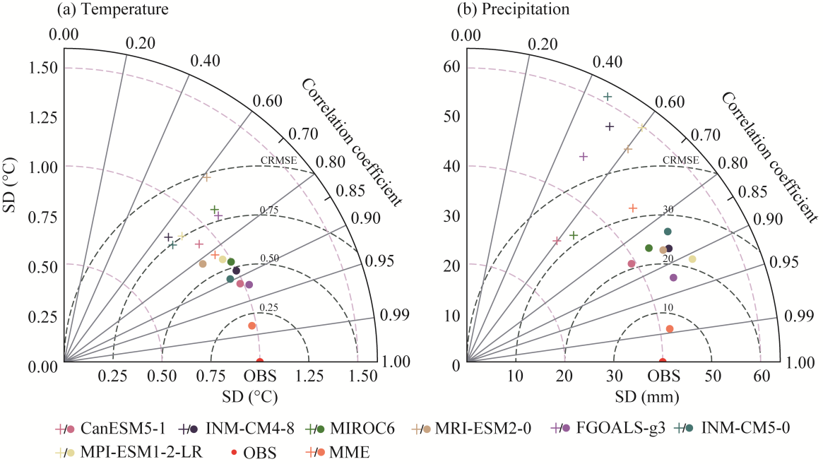
Fig. 2 Taylor diagrams for temperature (a) and precipitation (b) after deviation correction for the single and ensemble modes. Filled circles denote bias-corrected simulations, whereas "+" markers indicate raw simulations before bias correction. CRMSE, centered root mean square error; OBS, observation (reference dataset); MME, multi-model ensemble; SD, standard deviation.
With respect to precipitation, the raw simulations prior to correction show low agreement with the observations, with correlation coefficients of 0.47-0.73 (MME: 0.73), dispersed variability (SDs of 30.872-61.341 mm), and CRMSE values of 31.418-55.924 mm (Fig. 2b). After bias correction, the correlation coefficients range from 0.84 to 0.93, indicating improved agreement with the observations across the models. The SDs range from 39.135 to 50.622 mm, which are broadly consistent with the observations, whereas the CRMSE ranges from 12.349 to 28.695 mm. The MME again shows the closest agreement with the observations across the three Taylor diagram metrics.
The MME strongly agrees with the station observations across all variables at the daily scale, meeting or exceeding the typical performance thresholds reported in the CMIP6 evaluation studies (Table 5). Specifically, precipitation and temperature strongly agree with the observations (PBIAS=5.62% and 5.21%, respectively; RMSE=0.391 mm and 1.999°C, respectively; and NSE=0.9103 and 0.9695, respectively), suggesting minimal systematic bias and high fidelity in reproducing observed variability. Relative humidity and wind speed also perform well (PBIAS=0.33% and 8.10%, respectively; and NSE=0.7471 and 0.6893, respectively), although minor discrepancies in local variability between the simulations and observations persist. Solar radiation exhibits reasonable accuracy (PBIAS=11.83% and NSE=0.6876), which is consistent with the expected uncertainty ranges associated with subgrid atmospheric processes and cloud-aerosol interactions.
Table 5 Performance evaluation of the multi-model ensemble (MME)-simulated daily meteorological variables
Variable Percent bias (PBIAS; %) Root mean square error (RMSE) Nash-Sutcliffe efficiency (NSE)
Precipitation 5.62 0.391 mm 0.9103
Temperature 5.21 1.999°C 0.9695
Relative humidity 0.33 7.58% 0.7471
Wind speed 8.10 1.23 m/s 0.6893
Solar radiation 11.83 27.3 W/m2 0.6876
In summary, the MME outperforms the individual models and shows the highest overall agreement with the observed climate variables. This finding supports the use of an ensemble approach to reduce individual-model biases and enhance the robustness of climate inputs. Therefore, we used the MME to provide a more robust climate forcing for the SZI calculation and subsequent drought analyses in the basin.

3.2 Validation of the SZI with the observed NDVI

The deseasonalized scatter between the NDVI and SZI anomalies, together with a linear fit and a LOESS curve, is shown in Figure 3a. Both correlation metrics indicate a modest yet statistically robust positive association at zero lag (Pearson r=0.286; Spearman ρ=0.316; both P<0.001), indicating that departures toward wetter-than-normal conditions (high SZI anomalies) are generally accompanied by greener-than-normal vegetation states (high NDVI anomalies) after shared seasonality is removed. The LOESS curve suggests a largely monotonic relationship, with only limited curvature over the observed anomaly range.
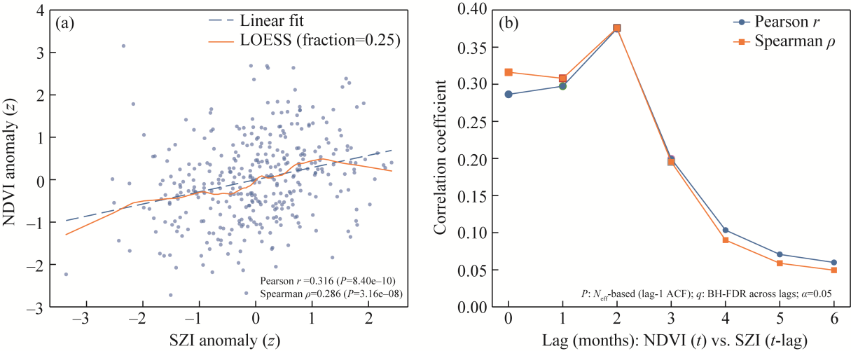
Fig. 3 Scatterplot of calendar-month standardized anomalies (z anomalies) between the basin-mean normalized difference vegetation index (NDVI) and standardized moisture anomaly index (SZI; a) and lagged correlations between NDVI (t) and SZI (t lag) for lags of 0-6 months (b) during 1985-2014. LOESS, locally estimated scatterplot smoothing; ACF, autocorrelation function; qFDR, Benjamini-Hochberg false discovery rate (BH-FDR) adjusted q-values.
Lagged results indicate that the association is strongest when the NDVI lags the SZI by almost 2 months (r=0.375; ρ=0.376; and both P<0.001 and qFDR<0.001), which is consistent with a delayed vegetation response to antecedent moisture availability (Fig. 3b; Table 6). The associations remain statistically supported up to a 3-month lag (r=0.200; ρ=0.195; and both P<0.001 and qFDR<0.001) but weaken thereafter. After accounting for multiple lags, correlations at lags≥4 are not robust, suggesting that the detectable NDVI-SZI association is confined primarily to a 0-3 month window, with the strongest linkage occurring at almost 2 months.
Table 6 Autocorrelation- and multiplicity-controlled lagged correlations between normalized difference vegetation index (NDVI) and SZI anomalies
Lag Pearson r Neff-based autocorrelation-adjusted P-value Spearman ρ Benjamini-Hochberg false discovery rate (BH-FDR) adjusted q-value (qFDR)
0 0.286 <0.001 0.316 <0.001
1 0.297 <0.001 0.308 <0.001
2 0.375 <0.001 0.376 <0.001
3 0.200 <0.001 0.195 <0.001
4 0.103 <0.001 0.090 0.165
5 0.071 0.220 0.059 0.359
6 0.060 0.298 0.049 0.390
Collectively, the anomaly based analysis with autocorrelation and multiple-testing controls provides an ecologically grounded consistency check: basin-scale SZI variability is mirrored in vegetation greenness anomalies, and the relationship exhibits a physically plausible short lag rather than spurious seasonality.

3.3 Temporal characteristics of drought

3.3.1 Anomaly characteristics of precipitation-evapotranspiration balance

The percentages anomalies of the annual precipitation minus the PET in the Weigan River Basin are shown in Figure 4 for 1970-2100. A comparative analysis for 2015-2100 reveals coherent scenario-dependent trends superimposed on substantial interannual variability.
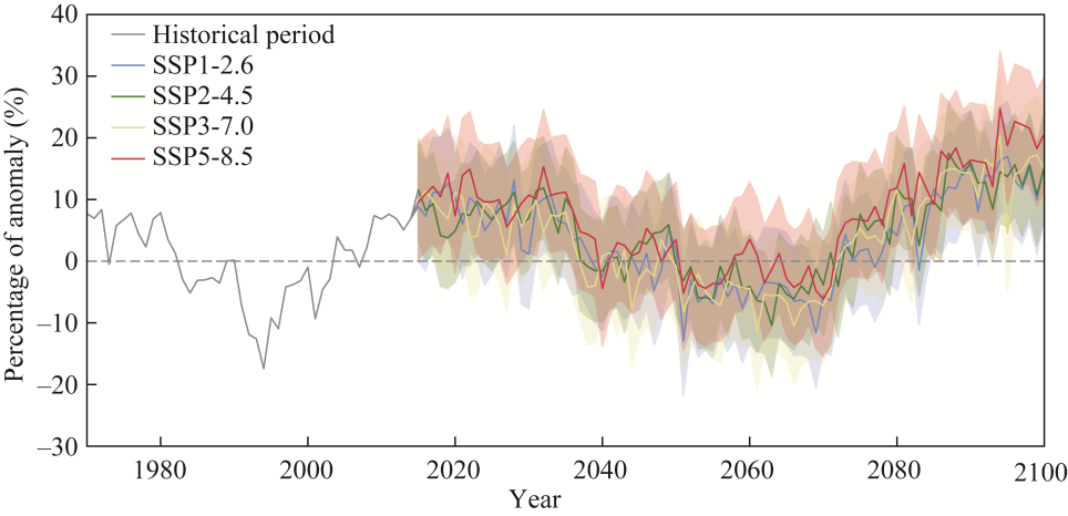
Fig. 4 Anomaly percentages representing the differences between annual precipitation and potential evapotranspiration (PET) in the Weigan River Basin from 1970 to 2100. The shaded envelopes indicate SD. SSP, shared socioeconomic pathway.
In terms of extremes, SSP5-8.5 has the greatest amplitude, with a maximum of 24.77% in 2094 and a minimum of -6.16% in 2070, yielding a total range of 30.94%. This large excursion indicates a strong perturbation of the moisture-balance anomaly under high-emission forcing relative to background variability. In contrast, SSP1-2.6 has a smaller extreme range (23.14%), suggesting a relatively muted excursion.
For trend characterization, the period 2015-2100 was divided into 2015-2050 and 2051-2100. During 2051-2100, the ensemble-mean anomaly percentage increases across all scenarios (e.g., 0.5884%/a under SSP5-8.5), indicating an upward shift in the mean moisture-balance state. Despite this multidecadal increase in the ensemble mean, year-to-year variability remains substantial, and occasional negative anomalies persist (including under SSP5-8.5). Overall, the late-century period is characterized by an upward shift in the ensemble mean relative to background variability. During 2015-2050, most scenarios show a slight decline (SSP5-8.5: -0.3436%/a), which is consistent with a period when increasing evaporative demand may offset precipitation-related gains.
We applied a 5-a moving SD, yielding multi-year mean values of the annual 5-a moving SD of the precipitation-PET anomaly of 2.73%-2.98% across scenarios to quantify interannual variability. In addition, the ±1 SD envelopes span approximately 13.6%-15.5% across all scenarios, highlighting substantial ensemble spread.

3.3.2 Temporal evolution and trend breaks of the SZI

Across the four emission scenarios, the temporal evolution of the SZI exhibits scenario-dependent breakpoint structures (Fig. 5). In general, the low- and medium-emission scenarios (SSP1-2.6 and SSP2-4.5) show an increasing trend before the breakpoint followed by a declining trend afterward, whereas the high-emission scenarios (SSP3-7.0 and SSP5-8.5) are characterized by predominantly negative trends.
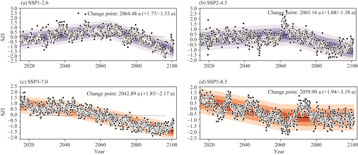
Fig. 5 Fitting diagram from the Bayesian piecewise regression model and interannual variation trend of the SZI under different scenarios in 2015-2100. (a), SSP1-2.6; (b), SSP2-4.5; (c), SSP3-7.0; (d), SSP5-8.5. Shaded areas indicate posterior predictive intervals at multiple credibility levels: the darkest shading corresponds to the 50.00% credible interval, intermediate shading represents the 80.00% credible interval, and the lightest shading denotes the 95.00% credible interval.
Under SSP1-2.6, a breakpoint is detected at approximately 2064.48 a (+1.77/-1.53 a). Before the breakpoint, the Ф1 interval is [0.511,0.666], indicating a significant positive trend, whereas after the breakpoint the Ф2 interval shifts to [-1.650, -1.397], indicating a significant negative trend.
A similar pattern is observed under SSP2-4.5, with a breakpoint at approximately 2065.16 a (+1.68/-1.38 a). The pre-breakpoint Ф1 interval of [0.174,0.316] indicates a significant positive trend, while the post-breakpoint Ф2 interval of [-1.261, -1.038] indicates a significant negative trend.
Under SSP3-7.0, the SZI displays a predominantly decreasing tendency throughout the study period. A breakpoint is identified at approximately 2042.89 a (+1.85/-2.17 a). Prior to the breakpoint, the Ф1 interval of [-1.888, -0.102] indicates a statistically significant drying trend. After the breakpoint, the Ф2 interval expands to [-0.905, 3.186], encompassing zero, suggesting that the post-breakpoint trend weakens and is no longer statistically significant. This indicates that the breakpoint reflects a change in the rate of drying rather than a reversal in trend direction. The SSP5-8.5 scenario exhibits the strongest drying signal among all pathways. A breakpoint is detected at approximately 2059.90 a (+1.94/-3.19 a). Prior to the breakpoint, the Ф1 interval of [-0.804, -0.656] confirms a statistically significant and persistent drying trend under strong external forcing. After the breakpoint, the Ф2 interval shifts to [-0.097, 0.072], which includes zero, indicating that the declining trend weakens and is no longer statistically significant.
Overall, the SZI trends differ significantly across the emission scenarios. Under SSP1-2.6 and SSP2-4.5, the region may experience a phase of humidification, whereas SSP3-7.0 and SSP5-8.5 are more likely to sustain or intensify drought conditions. Among these, SSP5-8.5 not only shows the most pronounced drying trend but is also associated with the greatest predictive uncertainty—highlighting that under high-emission scenarios, regional climate risks are elevated and system responses are more complex.

3.3.3 Tail dependence characteristics under extreme drought conditions

This study focused on two representative pathways: SSP2-4.5 and SSP5-8.5 to examine the statistical dependence and co-occurrence of extreme events in the SZI under different emission scenarios. These two scenarios were selected to represent a medium-emission pathway and a high-emission pathway in the CMIP6 framework, respectively, thereby enabling a contrast between moderate and strong external forcing conditions and their implications for extreme-drought co-variability. A bivariate vine copula model was employed to analyze the statistical associations among the SZI indices.
The fitting results indicate that the optimal copula was the t-copula, with an estimated correlation coefficient of -0.23 and estimated degrees of freedom (df) almost 4.8, resulting in an AIC value of -299.59. These results demonstrate that the model exhibits a good fit and effectively captures the dependence structure. The estimated correlation coefficient reflects overall dependence in the pseudo-observation space, indicating a weak negative association.
The joint-density contour plot in Figure 6 shows elevated density in the lower-left quadrant of the pseudo-observation space, corresponding to concurrent extreme dry states under SSP2-4.5 and SSP5-8.5. This pattern indicates moderate lower-tail dependence (tail co-variability) between the two SZI series under extreme-dry conditions. The estimated lower-tail dependence coefficient is 0.271, indicating moderate asymptotic lower-tail dependence, i.e., a tail association that remains nonzero as conditions become increasingly dry. The lower-tail dependence coefficient λL should be interpreted as an asymptotic tail-dependence measure rather than a discrete event probability. This indicates a nonnegligible co-extremal tendency in the extreme-dry tail of the two scenario series, without implying a fixed probability for any specific drought event. Overall, λL=0.271 suggests scenario-consistent extreme co-variability between SSP2-4.5 and SSP5-8.5 within the CMIP6 framework. Because both series are derived from the same multi-model CMIP6 framework and share externally forced and low-frequency components, part of this tail dependence may reflect common forcing and/or model structure.
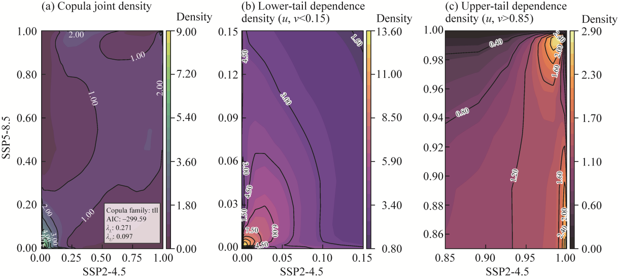
Fig. 6 Two-dimensional vine copula model results from the copula joint density (a), lower-tail dependence density for u, v<0.15 (b), and upper-tail dependence density for u, v>0.85 (c) between SSP2-4.5 and SSP5-8.5. tll denotes a Student's t copula with nonzero lower- and upper-tail dependence. AIC, Akaike information criterion; u and v, pseudo-observations (uniform margins) used in copula modeling; λL, lower-tail dependence coefficient; λU, upper-tail dependence coefficient.
In contrast, the upper-tail dependence coefficient is weak (λU=0.097), indicating weak to negligible upper-tail dependence; therefore, wet-tail behavior is not emphasized in the subsequent interpretation.

3.3.4 Contributions of precipitation and PET anomalies to historical SZI variability

We regressed the basin-mean monthly SZI on calendar-month-standardized anomalies of precipitation and PET for 1970-2014 to quantify the relative roles of water supply and atmospheric evaporative demand in shaping SZI variability. Both predictors are statistically significant (P<0.001), indicating that SZI variability reflects a coupled water-energy signal that is jointly associated with precipitation and PET anomalies rather than a precipitation-only signal. Given the substantial PET contribution, we explicitly account for PET-related sensitivity when we interpret seasonal changes in SZI-based drought frequency and trends (Fig. 7; Table 7). At the monthly scale, the standardized coefficients are comparable (0.419 for precipitation and 0.359 for PET), and the full model explains 58.16% of the variance in the SZI (R2=0.582).
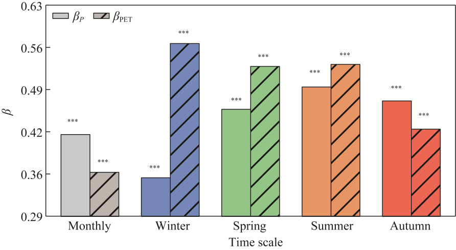
Fig. 7 Standardized regression coefficients of precipitation (βP) and PET (βPET) anomalies for explaining historical SZI variability at the monthly and seasonal scales during 1970-2014. β, standardized regression coefficient; ***, significance at P<0.001 level.
Table 7 Monthly and seasonal regression results for basin-mean SZI with precipitation and potential evapotranspiration (PET) anomalies during 1970-2014
Scale βP βPET R2
Monthly 0.419*** 0.359*** 0.582
Winter 0.351*** 0.561*** 0.649
Spring 0.458*** 0.525*** 0.603
Summer 0.493*** 0.528*** 0.490
Autumn 0.471*** 0.427*** 0.579

Note: βP, standardized regression coefficient for precipitation; βPET, standardized regression coefficient for PET; ***, statistical significance at P<0.001 level.

Seasonal regressions further reveal pronounced seasonality in these relative contributions. PET anomalies exert the strongest influence in winter (βP=0.351 vs. βPET=0.561; R2=0.649), whereas precipitation anomalies contribute strongly in spring and summer, and PET contribution weakens in autumn. These results provide an empirical basis for interpreting subsequent SZI-based analyses of drought frequency and trends, particularly in seasons when PET-related variability is substantial.

3.3.5 Changes in drought frequency and intra-annual seasonal distribution

The monthly and seasonal frequencies of moderate or more severe drought events that were identified using run theory under both historical and future climate scenarios are compared in Figure 8.
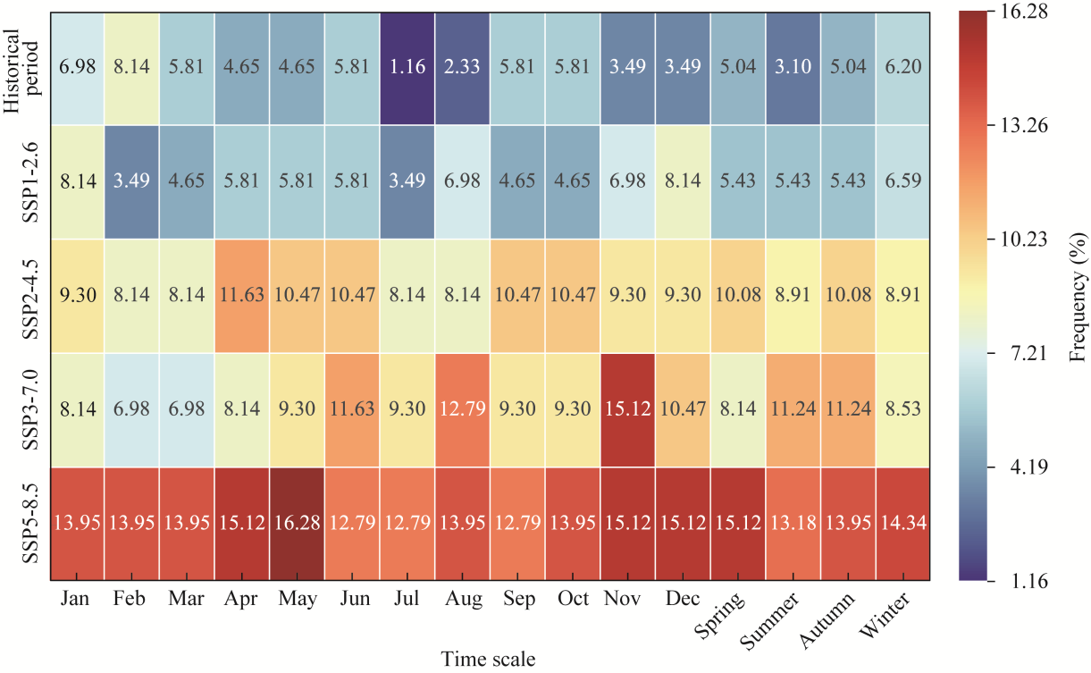
Fig. 8 Monthly and seasonally frequency of moderate and above drought events
During 1970-2014, drought event frequencies are relatively low in July and August, with July having the lowest annual frequency at only 1.16% (Fig. 7). However, in all future scenarios, the drought frequency increases notably, especially under SSP3-7.0 and SSP5-8.5. Under these scenarios, the July drought frequency increases to 9.30% and 12.79%, respectively, indicating a pronounced trend toward intensified summer drought in the future. Given the substantial contribution of PET to summer SZI variability, the projected increase in summer drought frequency indicated by the SZI is interpreted as a coupled precipitation-evaporative-demand signal rather than a precipitation-only change.
In terms of intra-annual variation, the SSP5-8.5 scenario consistently exhibits monthly drought frequencies that are higher than those in the other scenarios, peaking at 16.28% in May. In contrast, the historical scenario indicates a drought frequency of only 4.65% in May, suggesting that this month may become a critical period of elevated drought risk under high-emission pathways.
Moreover, the drought frequencies in October and November increase from 9.30% to 15.12% under SSP3-7.0 and from 13.95% to 15.12% under SSP5-8.5—well above the historical values of 5.81% and 3.49%, respectively. This finding suggests that in future scenarios, drought events may increasingly occur later in the year, resulting in autumn being another peak season for drought incidence, and that the seasonal distribution of droughts is expected to become more uniform.

3.4 Spatial characteristics of drought

3.4.1 Global spatial autocorrelation of drought duration

A global Moran's I spatial autocorrelation analysis was performed on drought duration under both historical (1970-2014) and future SSP scenarios, with the results summarized in Table 8. The analysis was conducted on the gridded drought duration fields at 0.250°, and Moran's I is therefore interpreted as clustering at this analysis support scale. Across all scenarios, the Moran's I values are significantly positive, ranging from 0.837 to 0.877, with Z scores between 279.51 and 292.33 (P<0.001). These results indicate that the spatial autocorrelation of drought duration is statistically significant, indicating that drought duration exhibits spatially coherent clustering rather than a random pattern in both the historical and projected scenarios.
Table 8 Results of spatial autocorrelation analysis in the Weigan River Basin under different scenarios
Historical period SSP1-2.6 SSP2-4.5 SSP3-7.0 SSP5-8.5
Moran's I 0.877 0.841 0.837 0.865 0.859
Z score 292.33 280.79 279.51 288.22 286.53
P <0.001 <0.001 <0.001 <0.001 <0.001

Note: SSP, shared socioeconomic pathway. Z score is the standardized test statistic associated with Moran's I under a normal approximation.

In comparison, the historical scenario exhibits the highest Moran's I value, suggesting that past drought durations show the strongest spatial coherence and clustering. In contrast, under the future SSP1-2.6 and SSP2-4.5 scenarios, spatial autocorrelation values are relatively low, implying that droughts may exhibit relatively weaker spatial clustering compared to the historical period under low- and medium-emission pathways. Conversely, under high-forcing scenarios such as SSP3-7.0 and SSP5-8.5, the Moran's I values increase to 0.865 and 0.859, respectively. This renewed clustering suggests that under more extreme climate conditions, drought-prone areas may become relatively more concentrated and potentially expand.
Overall, drought duration exhibits significant spatial clustering across all scenarios, underscoring that its regional pattern reflects spatially coherent hydroclimatic gradients and underlying physiographic controls (e.g., topography, hydrology, and land cover). Notably, the absolute magnitude of Moran's I can vary with spatial resolution and gridding choice; however, the consistently positive and significant values across scenarios robustly indicate nonrandom clustering in the drought duration field.

3.4.2 Spatially significant clustering of drought duration

The spatial distributions of statistically significant clustering in terms of drought duration across the Weigan River Basin during the historical period and under the four SSP scenarios are shown in Figure 9. Distinct hot spots (high-high clustering) and cold spots (low-low clustering) are consistently observed across all scenarios, indicating a persistent and spatially coherent aggregation pattern in terms of drought duration.
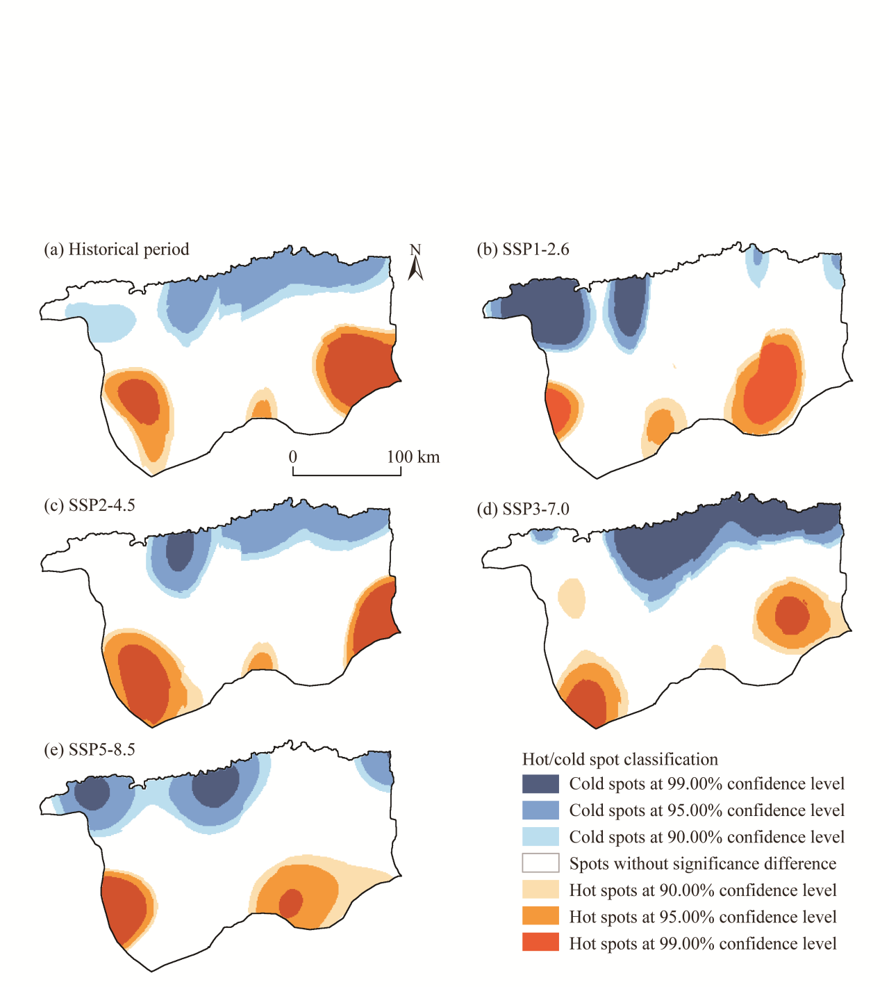
Fig. 9 Spatially aggregated significance distribution of drought duration in the Weigan River Basin from the Getis-Ord ${\text{G}}_{i}^{\text{*}}$ analysis for the historical period (a) and future scenarios SSP1-2.6 (b), SSP2-4.5 (c), SSP3-7.0 (d), and SSP5-8.5 (e)
The hot spots are concentrated mainly in the southern and southeastern basins, whereas the cold spots are distributed primarily in the northern sector, indicating strong spatial continuity across the scenarios. To quantify scenario-to-scenario differences, Table 9 summarizes the area and fractional coverage of statistically significant hot/cold spots, together with deviations from the historical reference and persistence metrics. Relative to the historical period (hot spot: 5760.72 km2 and 13.34%; and cold spot: 6538.32 km2, and 15.15%), SSP1-2.6 and SSP3-7.0 show expanded hot spot coverage (ΔF sig=+4.21 pp and +3.12 pp, respectively), whereas SSP5-8.5 exhibits a slight contraction (ΔF sig= -1.30 pp). In contrast, the number of cold spots increases substantially under SSP5-8.5 (9361.98 km2 and 21.72%; ΔF sig=+6.58 pp), indicating a pronounced expansion of statistically significant low-duration clustering under the highest forcing pathway.
Table 9 Quantification of statistically significant drought-duration hot spots/cold spots and their persistence across scenarios
Scenario Type A sig (km2) F sig (%) ΔF sig (pp) O HIS O Scen Jaccard
Historical period Hot spot 5760.72 13.34 0.00
Cold spot 6538.32 15.15 0.00
SSP1-2.6 Hot spot 7566.21 17.56 4.21 0.349 0.266 0.178
Cold spot 6268.59 14.55 -0.60 0.449 0.468 0.297
SSP2-4.5 Hot spot 5806.89 13.48 0.13 0.593 0.588 0.419
Cold spot 5991.57 13.90 -1.24 0.544 0.593 0.396
SSP3-7.0 Hot spot 7110.99 16.47 3.12 0.419 0.340 0.231
Cold spot 6598.26 15.28 0.13 0.384 0.381 0.236
SSP5-8.5 Hot spot 5188.86 12.04 -1.30 0.188 0.209 0.110
Cold spot 9361.98 21.72 6.58 0.652 0.456 0.367

Note: A sig is the total area of statistically significant cells (Z≥1.65 for hot spots and Z≤ -1.65 for cold spots) of the specified type within the basin; F sig is the corresponding fraction of the basin area (computed over valid basin cells); ΔF sig is the change in fraction relative to the historical baseline, expressed in percentage points (pp); O HIS is the overlap fraction of the historical mask retained in the scenario (intersection area divided by historical significant area); O Scen is the overlap fraction of the scenario mask covered by the historical mask (intersection area divided by the scenario significant area); and Jaccard is the Jaccard similarity index (intersection/union) between historical and scenario masks.

The results of the persistence analysis further indicate that the spatial overlap between the historical and future patterns varies by scenario. For hot spots, overlap with the historical pattern decreases markedly under SSP5-8.5 (O HIS=0.188 and Jaccard=0.110), suggesting reduced spatial persistence of high-duration clustering, whereas SSP2-4.5 is relatively more stable (O HIS=0.593 and Jaccard=0.419). With respect to the cold spots, the persistence remains relatively stronger, particularly under SSP5-8.5 (O HIS=0.652 and Jaccard=0.367). Collectively, these metrics complement the maps by demonstrating not only the visual continuity of the southern/southeastern hot spot zone and the northern cold spot belt but also the scenario-dependent magnitude of shifts in area and the degree of spatial persistence across emission pathways.

3.4.3 Identification of dominant factors driving drought hot spots on the basis of random forest

To characterize the environmental signatures associated with the spatial pattern of drought hot spots, we applied a random forest classifier to relate hot spot occurrence ( ${\text{G}}_{i}^{\text{*}}$ hot spot classes, Z≥1.96) to multisource geospatial predictors, including land use type, soil type (solonchak, gypsisol, fluyisol, gleysol, leptosol, chernozem, arenosol, anthrosol, phaeozem, and vertisol), DEM, slope, precipitation, PET, and soil moisture. Random forest was used here as an association-based pattern-attribution framework to quantify statistical linkages between hot spot occurrence and environmental gradients rather than to infer independent causality. We used SHAP to quantify each predictor's contribution to the random forest model output under each scenario to enhance interpretability.
The SHAP beeswarm plots for the historical period and four SSP scenarios are shown in Figure 10. Across scenarios, a consistent first-order structure is evident: the DEM and the hydroclimatic variables (precipitation, PET, and soil moisture) dominate the SHAP attribution, with the slope exerting a secondary but persistent contribution. In terms of the importance of the SHAP (mean |SHAP|), meteorological variables (precipitation and PET) account for 33.82%-44.57% across all scenarios, whereas topography (DEM and slope) contributes 26.51%-30.34%, and soil moisture alone accounts for an additional 15.49%-23.66%. This stability indicates that the hot spot pattern is jointly organized by climatic aridity gradients, terrain constraints, and land-surface water availability, with scenario-dependent changes primarily reflected in the relative weights among these leading controls.
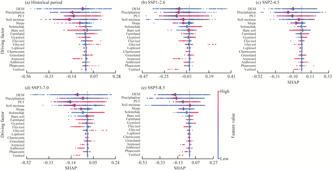
Fig. 10 Scenario-wise Shapley Additive exPlanations (SHAP) beeswarm plots of feature attributions for drought hot spot patterns from the random forest classifier (RFC) for the historical period (a) and future scenarios SSP1-2.6 (b), SSP2-4.5 (c), SSP3-7.0 (d), and SSP5-8.5 (e). For clarity, only the top 18 features ranked by mean absolute SHAP values are shown in each panel.
Among the individual predictors, DEM remains the most influential variable in all scenarios (mean |SHAP|=0.073-0.157), highlighting that hot spot occurrence is strongly structured along elevation-linked hydroclimatic and geomorphic gradients. SHAP attributions further show that precipitation and PET consistently make large contributions (mean |SHAP| for precipitation=0.054-0.148 and for PET=0.066-0.123), which is consistent with the statistical role of water supply-demand imbalance in shaping hot spot probability. Soil moisture also exhibits a robust contribution under all scenarios (mean |SHAP|=0.059-0.129), underscoring its relevance as an integrative state variable that links atmospheric conditions to near-surface moisture dynamics and drought persistence.
With respect to underlying surface properties, land use and soil type categories contribute less than the leading climatic-topographic controls to global SHAP attribution, yet several classes display nonnegligible and scenario-consistent signals. Bare soil and farmland repeatedly appear among the highest-ranked land use categories (e.g., historical mean |SHAP|=0.032 for bare soil and 0.016 for farmland; SSP2-4.5 mean |SHAP|=0.031 for bare soil and 0.018 for farmland), indicating that these surfaces are systematically associated with drought hot spot occurrence. Across all future climate scenarios, farmland consistently emerges as a hot spot region of drought impacting and facing elevated exposure to climate risk. In addition, the soil class solonchaks show relatively strong SHAP attribution in several future pathways (e.g., mean |SHAP|=0.032 under SSP1-2.6, 0.052 under SSP3-7.0, and 0.042 under SSP5-8.5), suggesting that saline soil environments are closely aligned with hot spot occurrence under projected climate conditions.
Overall, the random forest-SHAP results provide a coherent and scenario-robust attribution of the spatial pattern of drought hot spots: hot spot occurrence is statistically organized by elevation-linked gradients, hydroclimatic conditions (precipitation and PET), and soil moisture status, with land use/soil type classes modulating this pattern locally.

3.4.4 Spatial uncertainty analysis of drought

In this study, spatial DU was quantified by computing the pixelwise SD of drought hot spot classifications across multiple climate scenarios. A high SD indicates high variability in category assignments across scenarios, reflecting increased inter-scenario disagreement in projected drought patterns.
We conducted a correlation-matrix analysis between DUs and a set of topographic, climatic, soil moisture, and land use variables to explore potential associations with spatial uncertainty.
As shown in Figure 11, the correlations between DU and most natural factors were generally weak (|r|<0.050), suggesting that traditional environmental drivers have limited explanatory power for the spatial variability in drought prediction uncertainty. This pattern implies that the spatial variability in DU may primarily reflect structural differences across scenario-based climate model projections rather than being strongly constrained by the tested geographic or meteorological factors.
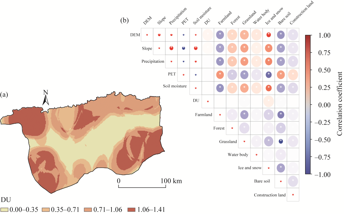
Fig. 11 Spatial distribution of drouth uncertainty (DU; a) and Pearson correlation matrix between DU and potential driving factors (b) across the Weigan River Basin. The magnitude of the ellipse reflects the strength of the relationship; large ellipses imply strong correlations. Blue ellipses denote negative correlations, whereas red ellipses indicate positive correlations. *, statistical significance at P<0.05 level.
Spatial overlays further reveal that areas with relatively high DUs tend to co-locate with topographically complex terrain and land use transition zones. However, given the uniformly weak DU-factor correlations (|r|<0.050), this colocation is interpreted as a qualitative spatial coincidence rather than evidence that landscape heterogeneity is a dominant driver of model divergence. In contrast, strong intercorrelations are observed among hydroclimatic factors (e.g., precipitation, PET, and soil moisture), which is consistent with theoretical expectations (|r|>0.800).
Among the tested factors, the highest DU correlation is with ice-snow cover (r=0.042, P<0.001), suggesting only a marginal association with spatial heterogeneity in hot- and cold-spot patterns under drought conditions. However, all the DU correlations are less than 0.050, indicating that no single factor provides a dominant linear explanation for the spatial pattern of DU.
Beyond DU, several strong intervariable relationships are evident. For instance, DEM is significantly positively correlated with precipitation (r=0.815, P<0.001) and soil moisture (r=0.883, P<0.001) and strongly negatively correlated with PET (r= -0.915, P<0.001). These relationships reflect elevation-linked hydroclimatic gradients across the basin. Soil moisture and PET are strongly negatively correlated (r= -0.975), and both are strongly correlated with precipitation, highlighting the strong coupling among key components of the basin water balance.
Among the land use categories, grassland is significantly negatively correlated with bare soil (r= -0.623), suggesting potential land cover differences and conversion dynamics. In contrast, construction land shows weak or negligible correlations with most natural variables. These findings indicate that DU is only weakly linearly associated with the tested natural and land-surface variables, whereas other variable pairs (elevation-climate linkages and land cover contrasts) exhibit strong relationships that reflect underlying ecological and topographic gradients. Accordingly, the spatial structure of DUs is more plausibly interpreted as reflecting inter-model structural differences and uncertainty propagation across scenarios rather than being directly controlled by any single landscape factor measured here.

4 Discussion

4.1 Consistency of the MME performance and ecological plausibility of the SZI

The magnitudes of the MME errors relative to the station observations are broadly consistent with those reported in recent CMIP6 evaluation studies, where temperature is typically simulated more robustly than precipitation and other hydroclimatic variables, and ensemble means reduce individual-model errors (Xu et al., 2021; Lei et al., 2023). This performance supports the use of the bias-corrected MME as a pragmatic basis for computing the SZI and comparing scenario-dependent drought characteristics in the basin. Moreover, the observed NDVI-SZI coupling, with peak associations occurring at 1-3 month lags, aligns with commonly reported vegetation response times to antecedent moisture anomalies in arid ecosystems (Zhong et al., 2021; Huang et al., 2024).

4.2 Physical basis and uncertainty bounds of SZI-based drought projections

SZI is adopted here as a physically informed drought metric embedded in a water-energy balance framework, and the index is designed to represent standardized moisture anomalies while explicitly accounting for both precipitation supply and atmospheric evaporative demand (Zhang et al., 2015; Ayantobo and Wei, 2019). This formulation is particularly relevant for arid basins, where drought evolution is commonly governed by the joint variability of water input and evaporative demand rather than precipitation alone, which is consistent with the conceptual basis of PET-inclusive indices such as the SPEI (Vicente-Serrano et al., 2013; Scheff and Frierson, 2015; Milly and Dunne, 2016).
Our results further indicate that basin-mean SZI variability is significantly associated with both precipitation and PET anomalies, with clear seasonality in their relative contributions. This finding supports the interpretation of SZI changes as a coupled "supply-demand" hydroclimatic signal. Moreover, PET sensitivity remains an important consideration in hyperarid settings because PET depends on both the chosen formulation and meteorological inputs (e.g., radiation, humidity, and wind), and these choices can influence long-term water balance diagnostics (Scheff and Frierson, 2015; Milly and Dunne, 2016).
Several additional sources of uncertainty delimit the confidence bounds of SZI-based projections. First, precipitation projections in arid Central Asia exhibit substantial scenario- and model-dependent spread, and CMIP6 precipitation projections over Xinjiang Uygur Autonomous Region also show marked inter-model dispersion; both can strongly affect regional drought diagnostics or projections that rely on simulated precipitation changes (Zhang et al., 2023; Zhao et al., 2023). Second, standardized drought indices often rely on distribution fitting; the choice of distribution and its tail behavior can influence estimated drought severity and frequency, especially for extremes (Vicente-Serrano et al., 2013; Stagge et al., 2015). Third, bias correction is frequently required for impact-oriented applications, but bias-adjustment approaches can differ in how well they preserve climate change signals, indicating the sensitivity of standardized indices to the chosen correction method (Teutschbein and Seibert, 2012; Cannon et al., 2015). Collectively, these factors do not invalidate the main conclusions, but they motivate emphasizing changes that are robust across the MME and reporting the ensemble spread alongside the ensemble means to better reflect projection uncertainty.

4.3 Physical interpretation of statistically detected breakpoints in the arid-basin moisture balance

The breakpoints detected in the scenario-dependent moisture-balance anomaly series are interpreted as reflections of shifts in the relative prominence of forced change versus internal variability at multidecadal scales rather than implying an abrupt regime shift at annual scales. In climate projections, apparent "change points" can emerge as the forced signal that progressively separates from the background variability (i.e., a time-of-emergence behavior), particularly under scenarios where radiative forcing and associated hydroclimatic responses evolve nonlinearly over time (Tebaldi et al., 2021).
For arid Central Asia, multidecadal changes in drought-relevant hydroclimate can arise from the combined effects of warming-driven increases in evaporative demand and circulation/moisture-transport changes that modulate precipitation and effective moisture. These interacting processes provide a physically consistent backdrop for the timing of statistically detected shifts in the precipitation-PET balance (Scheff and Frierson, 2015; Milly and Dunne, 2016; Zhao et al., 2023). Therefore, the detected breakpoints (e.g., the mid-to-late century shift under SSP2-4.5) are discussed as periods when the scenario-dependent forced tendency becomes more distinguishable relative to internal hydroclimatic variability at the basin scale.

4.4 Nonlinear dependence and robustness of extremes across scenarios

Although the overall association between the SZI series under SSP2-4.5 and SSP5-8.5 is relatively modest, the estimated lower-tail dependence (0.271) indicates a nonnegligible co-extremal tendency under extreme dry conditions. These results highlight that correlation-based measures may understate dependence in the tails, whereas tail-focused dependence metrics best reflect the co-occurrence structure during extremes (Serinaldi, 2013). Importantly, lower-tail dependence parameter should be interpreted as an asymptotic tail-dependence measure rather than a discrete event probability; it characterizes the persistence of dependence as conditions become increasingly dry.
A plausible interpretation is that part of this tail dependence reflects common external forcing and shared low-frequency variability embedded in the multi-model framework, which can promote more coherent behavior in the extreme-dry tail than in the wet tail. In dryland settings, drought extremes are also known to be associated with amplifying land-atmosphere feedback during hot and dry spells, which can contribute to coherence in extreme conditions across scenario realizations (Seneviratne et al., 2012). Accordingly, the detected asymmetric dependence structure supports the emphasis of robustness assessments for extremes using tail-sensitive diagnostics in addition to mean-trend comparisons.

4.5 Spatial persistence and interpretation of drought clustering patterns

The persistence of statistically significant hot/cold spots across scenarios suggests that drought duration is organized by a stable spatial association structure in the basin. It is also important to note that ${\text{G}}_{i}^{\text{*}}$ hot spot analysis evaluates statistically significant spatial clustering rather than the areal extent of drought-affected conditions: a scenario with more widespread drought can exhibit weak clustering significance if the spatial pattern becomes more diffuse or fragmented (Getis and Ord, 1992). This distinction helps explain why scenario-to-scenario differences in hot spot coverage and persistence do not necessarily mirror changes in the mean drought frequency or severity throughout the basin.
The southern/southeastern concentrations of hot spots and the northern cold spot zone remain visually coherent across scenarios, indicating that the spatial organization of drought duration is robust at the analysis scale. Therefore, scenario-dependent changes appear primarily as shifts in the magnitude and spatial persistence of clustering (rather than a wholesale relocation of the clustering structure), which is consistent with the combined influence of basin-scale hydroclimatic gradients and land-surface heterogeneity that can modulate where clustering becomes statistically pronounced.

4.6 Targeting farmland vulnerability in drought adaptation strategies

The pronounced vulnerability of farmland underscores the need for targeted drought adaptation strategies in agricultural areas. Given the region's critical role in supporting agricultural production and ecological security in the Tarim River Basin (Ke et al., 2020), future drought risk assessments and adaptation planning should explicitly prioritize farmland distribution and land use characteristics. An integrated approach—considering climatic variability, topographic conditions, and soil water-holding capacity—can support fine-scale drought monitoring and early warning to enhance agricultural resilience and water security planning (Meng et al., 2025).

4.7 Structural drivers and model inconsistencies in DU

Although no dominant driving factors were identified for DU, the analysis reveals strong internal couplings among key hydroclimatic and land-surface variables in the Weigan River Basin. In particular, soil moisture exhibits an extremely strong negative correlation with PET (r= -0.975), which is consistent with the strong land-atmosphere coupling reported in dryland environments (Dirmeyer, 2011). In addition, the significant negative correlation between grassland and bare soil (r= -0.623) is consistent with global evidence that vegetation cover enhances drought resilience relative to sparsely vegetated surfaces (Xiao et al., 2025). Importantly, these relationships describe the background structure of the hydroclimatic system, whereas the weak DU-factor correlations (|r|<0.050) indicate that DU itself is not well explained by any single landscape or climate variable in a linear sense. In this context, the observed spatial co-location between relatively high DU values and complex terrain or land use transition zones should be interpreted as qualitative coincidence rather than evidence of dominant landscape control. Therefore, the spatial pattern of DU values is more plausibly dominated by inter-model structural differences and uncertainty propagation within the CMIP6 MME, underscoring the need for future work to evaluate process representation and parameter sensitivity through process-based diagnostics and targeted sensitivity analyses.

5 Conclusions

In this study, future drought evolution in the Weigan River Basin was investigated using SZI derived from seven CMIP6 climate models under historical and four SSP scenarios. The results reveal that precipitation-evapotranspiration anomalies are projected to first decline but then increase over time, with increased fluctuations and uncertainty under high-emission scenarios. This phenomenon reflects intensified drought risks and the critical influence of emission trajectories on the regional water balance. Temporal analysis reveals that under low- and medium-emission scenarios, the SZI tends to shift from wetter to drier conditions, whereas high-emission scenarios are characterized by persistent drying and increased variability. A significantly lower-tail dependence was identified under extreme drought conditions (0.271), suggesting that extreme drought risks may be nonlinearly amplified across scenarios, even as general trends diverge. Moreover, the frequency of moderate and more severe drought events is expected to increase notably in the future, especially under SSP5-8.5, where drought is predicted to become more frequent year-round and expand into spring and autumn. Spatially, drought duration exhibits strong positive autocorrelation, with hot spots consistently located in the southern and southeastern basin and cold spots in the north. Random forest analysis, interpreted as association-based pattern attribution, indicates that precipitation and PET make the greatest contributions to the hot spot pattern, followed by topography and soil moisture. Farmland areas display high drought sensitivity across all scenarios, indicating the urgent need for adaptation strategies targeting agricultural regions. We developed a drought spatial uncertainty index by integrating hot spot patterns across the four future scenarios to assess scenario-driven spatial inconsistencies. The results indicate considerable spatial heterogeneity in DU, which is plausibly attributable to uncertainty propagation and inter-model structural differences within the CMIP6 MME. Key environmental gradients were identified, including topography-mediated hydroclimatic gradients and pronounced grassland-bare soil contrasts, reflecting the heterogeneity of the land-surface throughout the basin. These findings provide a scientific foundation for climate-resilient drought management and adaptive planning in arid inland basins.

Conflicts of interest

The authors declare that they have no known competing financial interests or personal relationships that could have appeared to influence the work reported in this paper.

Acknowledgements

This research was supported by the Key Research and Development Project of Xinjiang Uygur Autonomous Region, China (2022B02049) and the Major Science and Technology Special Project of Xinjiang Uygur Autonomous Region, China (2024A03007-5).

Author contributions

Conceptualization: WANG Wenbo; Methodology: WANG Wenbo; Software: WANG Wenbo; Validation: WANG Wenbo; Formal analysis: WANG Wenbo; Investigation: WANG Wenbo; Resources: LIN Li, WANG Wenbo; Data curation: WANG Wenbo, CHEN Dandan, YANG Jiayun; Writing - original draft preparation: WANG Wenbo; Writing - review and editing: WANG Wenbo; Visualization: WANG Wenbo; Supervision: LIN Li. All authors approved the manuscript.
[1]
Ayantobo O O, Wei J. 2019. Appraising regional multi-category and multi-scalar drought monitoring using standardized moisture anomaly index (SZI): a water-energy balance approach. Journal of Hydrology, 579: 124139, doi: 10.1016/j.jhydrol.2019.124139.

[2]
Behzadi F, Javadi S, Yousefi H, et al. 2024. Projections of meteorological drought severity-duration variations based on CMIP6. Scientific Reports, 14: 5027, doi: 10.1038/s41598-024-55340-x.

PMID

[3]
Brilleman S L, Howe L D, Wolfe R, et al. 2017. Bayesian piecewise linear mixed models with a random change point: an application to BMI rebound in childhood. Epidemiology, 28(6): 827-833.

DOI PMID

[4]
Cannon A J, Sobie S R, Murdock T Q. 2015. Bias correction of GCM precipitation by quantile mapping: how well do methods preserve changes in quantiles and extremes? Journal of Climate, 28(17): 6938-6959.

DOI

[5]
Ding X Y, Yu Y, Yang M L, et al. 2024. Investigating the effect of climate change on drought propagation in the Tarim River Basin using multi-model ensemble projections. Atmosphere, 15(1): 50, doi: 10.3390/atmos15010050.

[6]
Dirmeyer P A. 2011. The terrestrial segment of soil moisture-climate coupling. Geophysical Research Letters, 38(16): L16702, doi: 10.1029/2011GL048268.

[7]
Eyring V, Bony S, Meehl G A, et al. 2016. Overview of the Coupled Model Intercomparison Project Phase 6 (CMIP6) experimental design and organization. Geoscientific Model Development, 9(5): 1937-1958.

DOI

[8]
Getis A, Ord J K. 1992. The analysis of spatial association by use of distance statistics. Geographical Analysis, 24(3): 189-206.

DOI

[9]
Guo H, Jiapaer G, Bao A M, et al. 2017. MPDI-based comparison on spatiotemporal variation of drought over oasis and desert in Tarim Basin. Journal of Desert Research, 37(4): 775-783. (in Chinese)

[10]
Hanby G, Zhai L, Mishra B, et al. 2025. A comprehensive outlook on drought caused economic losses and landowner perceptions concerning drought and erratic rainfall patterns. Forest Policy and Economics, 170: 103405, doi: 10.1016/j.forpol.2024.103405.

[11]
Huang W W, Henderson M, Liu B H, et al. 2024. Cumulative and lagged effects: seasonal characteristics of drought effects on East Asian grasslands. Remote Sensing, 16(18): 3478, doi: 10.3390/rs16183478.

[12]
Ke Y M, Shen Z F, Bai J, et al. 2020. Analysis of suitable scale for cultivated land in the Ugan River Basin accounting for water resource constraints. Arid Zone Research, 37(3): 551-561. (in Chinese)

[13]
Lei X N, Xu C C, Liu F, et al. 2023. Evaluation of CMIP6 models and multi-model ensemble for extreme precipitation over arid Central Asia. Remote Sensing, 15(9): 2376, doi: 10.3390/rs15092376.

[14]
Li H B, Wang W G, Fu J Y, et al. 2023a. Spatiotemporal heterogeneity and attributions of streamflow and baseflow changes across the headstreams of the Tarim River Basin, Northwest China. Science of The Total Environment, 856: 159230, doi: 10.1016/j.scitotenv.2022.159230.

[15]
Li J, Bevacqua E, Wang Z L, et al. 2023b. Hydroclimatic extremes contribute to asymmetric trends in ecosystem productivity loss. Communications Earth & Environment, 4: 197, doi: 10.1038/s43247-023-00869-4.

[16]
Li Q Q, Ye A Z, Wada Y, et al. 2024. Climate change leads to an expansion of global drought-sensitive area. Journal of Hydrology, 632: 130874, doi: 10.1016/j.jhydrol.2024.130874.

[17]
Li S N. 2015. Analysis on evolvement characteristics of drought under changing environment in Aksu River Basin. MSc Thesis. Handan: Hebei University of Engineering. (in Chinese)

[18]
Liu J G, Yang H, Gosling S N, et al. 2017. Water scarcity assessments in the past, present, and future. Earth's Future, 5(6): 545-559.

DOI

[19]
Liu X Y, Li X M, Zhang Z R, et al. 2024. A CMIP6-based assessment of regional climate change in the Chinese Tianshan Mountains. Journal of Arid Land, 16(2): 195-219.

DOI

[20]
Meng X Y, Zhang S, Wang G Q, et al. 2025. Decoding agricultural drought resilience: a triple-validated random forest framework integrating multi-source remote sensing for high-resolution monitoring in the North China Plain. Remote Sensing, 17(8): 1404, doi: 10.3390/rs17081404.

[21]
Milly P C D, Dunne K A. 2016. Potential evapotranspiration and continental drying. Nature Climate Change, 6: 946-949.

DOI

[22]
Orimoloye I R, Belle J A, Ololade O O. 2021. Drought disaster monitoring using MODIS derived index for drought years: a space-based information for ecosystems and environmental conservation. Journal of Environmental Management, 284: 112028, doi: 10.1016/j.jenvman.2021.112028.

[23]
Pathak R, Dasari H P, Ashok K, et al. 2023. Effects of multi-observations uncertainty and models similarity on climate change projections. npj Climate and Atmospheric Science, 6: 144, doi: 10.1038/s41612-023-00473-5.

[24]
Scheff J, Frierson D M W. 2015. Terrestrial aridity and its response to greenhouse warming across CMIP 5 climate models. Journal of Climate, 28(14): 5583-5600.

DOI

[25]
Seneviratne S I, Nicholls N, Easterling D, et al. 2012. Changes in climate extremes and their impacts on the natural physical environment. In: Field CB, BarrosV, Stocker TF, et al. Managing the Risks of Extreme Events and Disasters to Advance Climate Change Adaptation. Cambridge: Cambridge University Press, 109-230.

[26]
Serinaldi F. 2013. An uncertain journey around the tails of multivariate hydrological distributions. Water Resources Research, 49(10): 6527-6547.

DOI

[27]
Soares P M M, Johannsen F, Lima D C A, et al. 2024. High-resolution downscaling of CMIP6 Earth system and global climate models using deep learning for Iberia. Geoscientific Model Development, 17(1): 229-259.

DOI

[28]
Stagge J H, Tallaksen L M, Gudmundsson L, et al. 2015. Candidate distributions for climatological drought indices (SPI and SPEI). International Journal of Climatology, 35(13): 4027-4040.

DOI

[29]
Tebaldi C, Debeire K, Eyring V, et al. 2021. Climate model projections from the Scenario Model Intercomparison Project (ScenarioMIP) of CMIP6. Earth System Dynamics, 12(1): 253-293.

DOI

[30]
Teutschbein C, Seibert J. 2012. Bias correction of regional climate model simulations for hydrological climate-change impact studies: review and evaluation of different methods. Journal of Hydrology, 456-457: 12-29.

DOI

[31]
Tian P Z, Jian B Y, Li J R, et al. 2023. Land-use-change-induced cooling and precipitation reduction in China: insights from CMIP 6 models. Sustainability, 15(16): 12191, doi: 10.3390/su151612191.

[32]
Vicente-Serrano S M, Gouveia C, Camarero J J, et al. 2013. Response of vegetation to drought time-scales across global land biomes. Proceedings of the National Academy of Sciences of the United States of America, 110(1): 52-57.

[33]
Wang H J, Chen Y N, Li W H, et al. 2013. Runoff responses to climate change in arid region of northwestern China during 1960-2010. Chinese Geographical Science, 23(3): 286-300.

DOI

[34]
Wang Q F, Zhang R R, Qi J Y, et al. 2022. An improved daily standardized precipitation index dataset for mainland China from 1961 to 2018. Scientific Data, 9: 124, doi: 10.1038/s41597-022-01201-z.

PMID

[35]
Wang T T. 2022. Study on potential evapotranspiration and drought characteristics in Tarim River Basin. MSc Thesis. Shanghai: Shanghai Normal University. (in Chinese)

[36]
Wu H J, Su X L, Singh V P, et al. 2021. Agricultural drought prediction based on conditional distributions of vine copulas. Water Resources Research, 57(8): e2021WR029562, doi: 10.1029/2021WR029562.

[37]
Xiang Y Y, Wang Y, Chen Y N, et al. 2024. Prediction of future hydrological drought risk in the Yarkant River Basin based on CMIP 6 models. Arid Land Geography, 47(5): 798-809. (in Chinese)

[38]
Xiao C W, Zaehle S, Sitch S, et al. 2025. Deforestation increases vegetation vulnerability to drought across biomes. Global Biogeochemical Cycles, 39(5): e2024GB008378, doi: 10.1029/2024GB008378.

[39]
Xu J W, Zhang X T, Feng C J, et al. 2021. Evaluation of surface upward longwave radiation in the CMIP6 models with ground and satellite observations. Remote Sensing, 13(21): 4464, doi: 10.3390/rs13214464.

[40]
Yang P, Xia J, Zhang Y Y, et al. 2019. How is the risk of hydrological drought in the Tarim River Basin, Northwest China? Science of The Total Environment, 693: 133555, doi: 10.1016/j.scitotenv.2019.07.361.

[41]
Zhai J Q, Mondal S K, Fischer T, et al. 2020. Future drought characteristics through a multi-model ensemble from CMIP 6 over South Asia. Atmospheric Research, 246: 105111, doi: 10.1016/j.atmosres.2020.105111.

[42]
Zhang B Q, Zhao X N, Jin J M, et al. 2015. Development and evaluation of a physically based multiscalar drought index: the standardized moisture anomaly index. Journal of Geophysical Research: Atmospheres, 120(22): 11575-11588.

[43]
Zhang G W, Zeng G, Yang X Y, et al. 2021a. Future changes in extreme high temperature over China at 1.5°C-5°C global warming based on CMIP 6 simulations. Advances in Atmospheric Sciences, 38(2): 253-267.

DOI

[44]
Zhang G X, Su X L, Singh V P, et al. 2021b. Appraising standardized moisture anomaly index (SZI) in drought projection across China under CMIP 6 forcing scenarios. Journal of Hydrology: Regional Studies, 37: 100898, doi: 10.1016/j.ejrh.2021.100898.

[45]
Zhang X L, Wang X X, Zhou B T. 2023. CMIP6-projected changes in drought over Xinjiang, Northwest China. International Journal of Climatology, 43(14): 6560-6577.

DOI

[46]
Zhao Z Y, Hao X M, Fan X, et al. 2023. Actual evapotranspiration dominates drought in Central Asia. Remote Sensing, 15(18): 4557, doi: 10.3390/rs15184557.

[47]
Zhong S B, Sun Z H, Di L P. 2021. Characteristics of vegetation response to drought in the CONUS based on long-term remote sensing and meteorological data. Ecological Indicators, 127: 107767, doi: 10.1016/j.ecolind.2021.107767.

[48]
Zhou T J, Zou L W, Chen X L. 2019. Commentary on the coupled model intercomparison project phase 6 (CMIP6). Climate Change Research, 15(5): 445-456. (in Chinese)

Outlines

/