Research article

Multi-source remote sensing and machine learning reveal spatiotemporal variations and drivers of NPP in the Tianshan Mountains, China

  • LI Jiani 1, 2, 3, 4 ,
  • XU Denghui 1, 2, 3, 4 ,
  • XU Zhonglin 1, 2, 3, 4 ,
  • WANG Yao , 1, 5, * ,
  • YANG Jianjun 1, 2, 3, 4
Expand
  • 1College of Ecology and Environment, Xinjiang University, Urumqi 830017, China
  • 2Key Laboratory of Oasis Ecology, Xinjiang University, Urumqi 830017, China
  • 3Xinjiang Jinghe Observation and Research Station of Temperate Desert Ecosystem, Ministry of Education, Urumqi 830017, China
  • 4Technology Innovation Center for Ecological Monitoring and Restoration of Desert-Oasis, Urumqi 830001, China
  • 5Institute of Desert Meteorology, China Meteorological Administration, Urumqi 830002, China
*WANG Yao (E-mail: )

Received date: 2025-09-25

  Revised date: 2025-12-25

  Accepted date: 2025-12-31

  Online published: 2026-02-04

Abstract

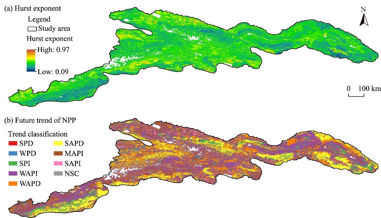
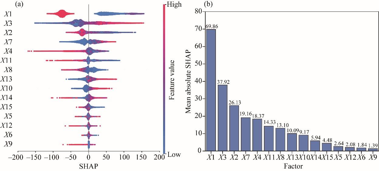
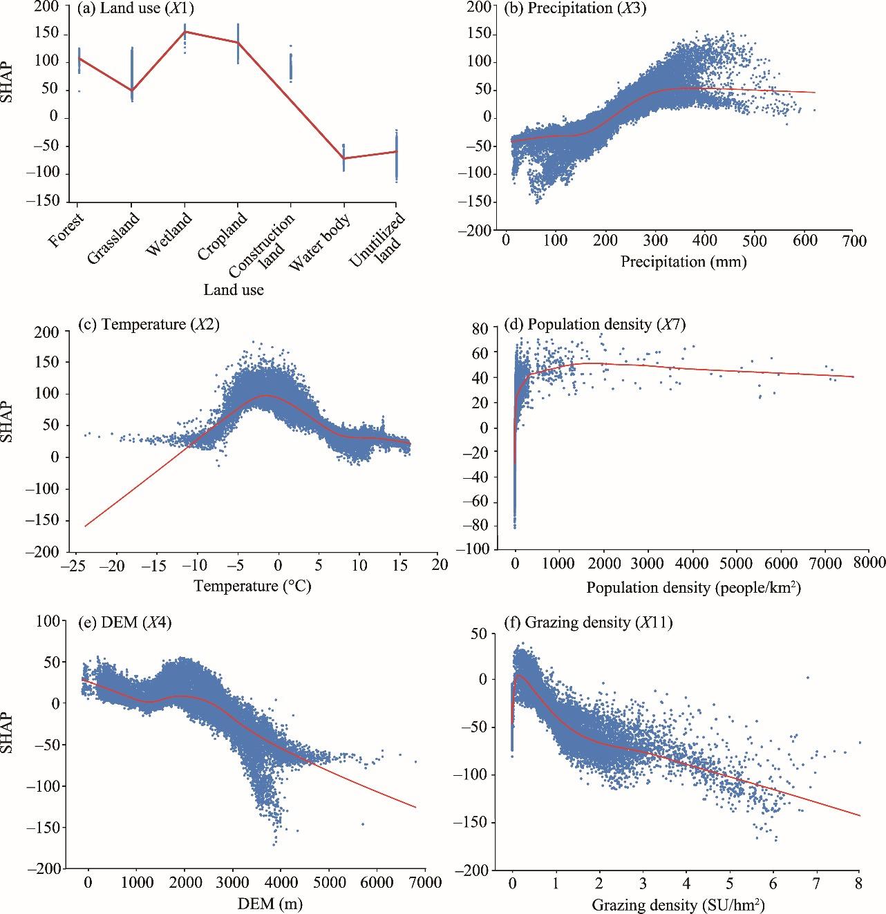
Arid mountain ecosystems are highly sensitive to hydrothermal stress and land use intensification, yet where net primary productivity (NPP) degradation is likely to persist and what drives it remain unclear in the Tianshan Mountains of Northwest China. We integrated multi-source remote sensing with the Carnegie-Ames-Stanford Approach (CASA) model to estimate NPP during 2000-2020, assessed trend persistence using the Hurst exponent, and identified key drivers and nonlinear thresholds with Extreme Gradient Boosting (XGBoost) and SHapley Additive exPlanations (SHAP). Total NPP averaged 55.74 Tg C/a and ranged from 48.07 to 65.91 Tg C/a from 2000 to 2020, while regional mean NPP rose from 138.97 to 160.69 g C/(m2•a). Land use transfer analysis showed that grassland expanded mainly at the expense of unutilized land and that cropland increased overall. Although NPP increased across 64.11% of the region during 2000-2020, persistence analysis suggested that 53.93% of the Tianshan Mountains was prone to continued NPP decline, including 36.41% with significant projected decline and 17.52% with weak projected decline; these areas formed degradation hotspots concentrated in the central and northern Tianshan Mountains. In contrast, potential improvement was limited (strong persistent improvement: 4.97%; strong anti-persistent improvement: 0.36%). Driver attribution indicated that land use dominated NPP variability (mean absolute SHAP value=29.54%), followed by precipitation (16.03%) and temperature (11.05%). SHAP dependence analyses showed that precipitation effects stabilized at 300.00-400.00 mm, and temperature exhibited an inverted U-shaped response with a peak near 0.00°C. These findings indicated that persistent degradation risk arose from hydrothermal constraints interacting with land use conversion, highlighting the need for threshold-informed, spatially targeted management to sustain carbon sequestration in arid mountain ecosystems.

Cite this article

LI Jiani , XU Denghui , XU Zhonglin , WANG Yao , YANG Jianjun . Multi-source remote sensing and machine learning reveal spatiotemporal variations and drivers of NPP in the Tianshan Mountains, China[J]. Journal of Arid Land, 2026 , 18(1) : 56 -83 . DOI: 10.1016/j.jaridl.2026.01.006

1 Introduction

Dryland areas have become a focal point of global-change research because warming-driven aridification and more frequent hydroclimatic extremes are reshaping ecosystem functioning, carbon uptake, and ecological security. These changes are critical for climate mitigation as well as for regional sustainability, given that semi-arid and arid ecosystems contribute disproportionately to the variability and long-term trend of the terrestrial carbon sink (Ahlström et al., 2015; Friedlingstein et al., 2023) and remain highly sensitive to water limitation (Huang et al., 2016; IPCC, 2021). In arid areas, oases embedded within mountain-desert systems act as ecological "lifelines", but their stability is increasingly challenged by coupled climatic stressors and rapid land use intensification, which has motivated renewed synthesis on oasis ecological security and sustainable development (Chen et al., 2024b).
The Tianshan Mountains in northwestern China are a representative mountain-desert-oasis complex system and a crucial "water tower" for Central Asia. Cryospheric meltwater, orographic precipitation, and strong elevational gradients jointly sustain mountain forests, grasslands, and downstream oases while also amplify the system's vulnerability to climate warming and human disturbance (Chen et al., 2016). Recent studies have documented pronounced spatial heterogeneity in vegetation change across the Central Asian Tianshan Mountains and emphasized the role of climatic differentiation and topographic constraints (Yin et al., 2016; Du et al., 2025; Ma et al., 2025a). Meanwhile, regional ecological-security assessments highlight that ecosystem services and risk patterns in the Tianshan Mountains are spatially structured and management-relevant (Chen et al., 2024a). These findings collectively underscore the need for spatially explicit diagnostics that can both characterize vegetation productivity dynamics and explain why "degradation-prone" areas emerge under coupled natural and anthropogenic drivers.
Net primary productivity (NPP) provides a core and process-related indicator of vegetation carbon assimilation and ecosystem functioning, and is widely used to monitor productivity changes under climate variability and anthropogenic pressure. Satellite-driven NPP estimation has advanced rapidly, ranging from Moderate Resolution Imaging Spectroradiometer (MODIS)-type production algorithms to light use efficiency approaches and their regional improvements (Turner et al., 2006; Guan et al., 2022). However, rugged terrain and strong microclimatic gradients in arid mountains can magnify uncertainties associated with meteorological forcing, land-cover classification, and scale mismatches, leading to nontrivial disagreement among NPP products and model outputs (Robinson et al., 2018). To address these issues, many studies have adopted or refined the Carnegie-Ames-Stanford Approach (CASA) model and related frameworks for regional applications (Abdi et al., 2016; Bao et al., 2016), including recent model improvements and large-scale implementations enabled by cloud-based platforms (Wu et al., 2022; Dong et al., 2025). Yet, in arid mountain-oasis systems, a persistent challenge remains: estimating long-term NPP dynamics in a way that is both robust to product uncertainty and directly informative for spatial management.
Attribution of NPP change is equally challenging. In dryland and mountain areas, NPP often responds nonlinearly to hydrothermal conditions due to threshold-like constraints in soil moisture, temperature, and vapor pressure deficit, while human activities can either offset or exacerbate climate impacts through land use conversion, irrigation, restoration programs, and infrastructure expansion (Chen et al., 2023; Liu et al., 2024). Conventional approaches (e.g., correlation analysis, linear regression, and residual-trend methods) have clarified broad climate versus human contributions in many settings, but they may underperform when driver interactions are strong, response curves are highly nonlinear, or multiple thresholds coexist across elevation and land-cover gradients. These limitations have motivated the adoption of machine learning models that can capture nonlinearities and interactions more flexibly. In particular, Extreme Gradient Boosting (XGBoost) has become popular for geoscience applications because it combines high predictive skill with scalability (Chen and Guestrin, 2016; Grekousis, 2025). More importantly, interpretability tools such as SHapley Additive exPlanations (SHAP) provide consistent and additive feature attributions that can reveal dominant drivers and response thresholds in a transparent manner, supporting mechanism-oriented inference rather than "black-box" prediction (Lundberg and Lee, 2017; Wu et al., 2024b).
Beyond explaining past changes, decision-making in fragile arid systems also requires an assessment of whether current trends are likely to persist. A growing body of remote-sensing studies has therefore combined trend analysis with persistence diagnostics (e.g., Hurst-based measures) to distinguish areas where vegetation trajectories are likely to continue, reverse, or fluctuate stochastically (Kalisa et al., 2019; Jiang et al., 2022). Similar logic has been applied to NPP to characterize potential future sustainability of productivity trends (Liang et al., 2025), and recent evidence suggests that "persistence" itself can differ systematically across hydroclimatic gradients and ecosystem types (Ren et al., 2025). However, in the Tianshan Mountains and comparable mountain-desert-oasis systems, few studies have tightly integrated long-term NPP estimation, persistence-oriented risk screening, and explainable machine learning for nonlinear attribution and threshold detection within one coherent framework. This integration is essential for identifying where "degradation hotspots" are most likely to emerge and which controllable drivers provide the greatest leverage for targeted interventions.
To fill these gaps, this study investigated spatiotemporal variations, persistence characteristics, and driving mechanisms of NPP in the Tianshan Mountains from 2000 to 2020. Specifically, the research first estimated annual NPP using a light use efficiency-based (CASA-type) framework supported by multi-source remote-sensing and climate data. Building on this foundation, we quantified NPP trends and persistence to identify areas prone to sustained decline versus improvement. To disentangle the driving mechanisms, we analyzed the relative importance of climatic and anthropogenic drivers using XGBoost, with their effects interpreted via absolute SHAP values to reveal nonlinear response patterns and thresholds. Ultimately, this study aimed to translate these integrated diagnostics into spatially explicit implications for ecological management in the mountain-desert-oasis complex system.

2 Materials

2.1 Study area

The Tianshan Mountains form the central mountain system of Xinjiang Uygur Autonomous Region, China (39°24′40″-45°23′08″N, 73°50′28″-95°33′56″E). This study focused on the Chinese sector, spanning 11 prefecture-level administrative units and covering about 37.02×10⁴ km2 (Fig. 1). The range has an average ridgeline elevation of about 4000 m, and Tomur Peak reaches 7443 m a.s.l. (Lu et al., 2022). The Tianshan Mountains form the natural and climatic divide between the Junggar Basin to the north and the Tarim Basin to the south, bordering the Taklimakan Desert and the Gurbantunggut Desert, and representing a typical mountain-oasis-desert complex system (Wang et al., 2016; Zhou and Lei, 2018). Climate conditions exhibit pronounced north-south contrasts: the annual mean temperature ranges from 2.50°C-5.00°C on the northern slope to 7.50°C-10.00°C on the southern slope (Li et al., 2019). Water scarcity is a defining feature, with strong spatial precipitation gradients: on the northern slope, annual precipitation decreases from approximately 250.00-350.00 mm in the western sector to 150.00-200.00 mm in the central sector, while the southern slope generally receives less precipitation than the northern slope (Wang et al., 2016). In the adjacent Tarim Basin, annual total precipitation is typically less than 50.00 mm, highlighting the hyper-arid background of the region (Zhou and Lei, 2018). As a "water tower of Central Asia", the Tianshan Mountains supply the headwaters of major regional rivers through combined contributions of glacier/snow meltwater and mountain precipitation (Chen et al., 2016). Their strong elevation gradients produce clear vertical zonation that supports diverse vegetation belts and ecosystem functions relevant to NPP dynamics in arid mountains (Li et al., 2019).
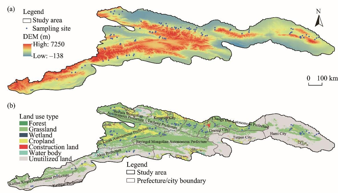
Fig. 1 Elevation (a) and land use type spatial distribution (b) in the Tianshan Mountains in Xinjiang Uygur Autonomous Region, China. DEM, digital elevation model.

2.2 Data collection and processing

This study assembled and preprocessed multi-source datasets to support the integrated analytical framework (Table 1). Core environmental variables included land use, the normalized difference vegetation index (NDVI), climatic and topographic factors, which served as the primary inputs to CASA model for estimating NPP. Monthly remote-sensing and meteorological data were used to drive CASA and to generate annual composites and cumulative values for the period 2000-2020. Anthropogenic pressure indicators included population density, gross domestic product (GDP) density, nighttime light index, human footprint, and grazing intensity, and accessibility metrics included distances to roads, highways, water bodies, and government centers; these variables were compiled to quantify anthropogenic pressure and infrastructure accessibility influences on NPP. Spatial consistency across datasets was ensured through reprojection, resampling to a 1-km resolution, and grid alignment. To refine the hydrothermal fields used by CASA, we complemented TerraClimate data with higher-resolution temperature and precipitation from the National Tibetan Plateau Data Center (NTPDC; https://data.tpdc.ac.cn/home). To represent land-cover classification uncertainty and recent changes, we jointly used two land-cover products: the Land Use and Cover Change (LUCC) dataset provided by Resource and Environmental Science Data Platform (http://www.resdc.cn) and the China Land Cover Dataset (CLCD) (https://zenodo.org/records/15853565). In addition, a 2024 data snapshot was compiled for supplementary near-term assessments and ongoing monitoring only and was not included in the core 2000-2020 analyses. All supplementary datasets used for robustness checks were harmonized to match the projection, spatial resolution, and grid of the core dataset.
Table 1 Data sources
Indicator Year Resolution Data source
Land use type 2000-2020 Annual, 500 m MCD12Q1 dataset (https://www.earthdata.nasa.gov/data/catalog/lpcloud-mcd12q1-061)
NDVI 2000-2020 Monthly, 1 km MOD13A3 dataset (https://www.earthdata.nasa.gov/data/catalog/lpcloud-mod13a3-061)
NPP (g C/(m2•a)) 2020 Annual,
1 km
MOD17A3 dataset (https://www.earthdata.nasa.gov/data/catalog/lpcloud-mod17a3hgf-061)
Solar radiation (W/m2) 2000-2020 Monthly, 4 km TerraClimate (https://climate.northwestknowledge.net/TERRACLIMATE/)
Temperature (℃) 2000-2020 Monthly, 4 km TerraClimate (https://climate.northwestknowledge.net/TERRACLIMATE/)
Precipitation (mm) 2000-2020 Monthly, 4 km TerraClimate (https://climate.northwestknowledge.net/TERRACLIMATE/)
DEM (m) 2020 Annual, 30 m Geospatial Data Cloud (https://www.gscloud.cn/)
Slope (°) 2020 Annual, 30 m Calculated by DEM
Aspect 2020 Annual, 30 m Calculated by DEM
Population density (persons/km2) 2020 Annual,
1 km
Resource and Environmental Science Data Platform (https://www.resdc.cn)
GDP density
(×104 CNY/km2)
2020 Annual,
1 km
Resource and Environmental Science Data Platform (https://www.resdc.cn)
Nighttime light index 2020 Annual,
1 km
Resource and Environmental Science Data Platform (https://www.resdc.cn)
Human footprint 2020 Annual,
1 km
Scientific data (https://doi.org/10.6084/m9.figshare.16571064)
Grazing intensity (SU/hm2) 2020 Annual,
1 km
Global Resource Data Cloud (https://www.gis5g.com/)
Distance to the road (km) 2020 OpenStreetMap (https://www.openstreetmap.org/)
Distance to highway (km) 2020 OpenStreetMap (https://www.openstreetmap.org/)
Distance to water body (km) 2020 OpenStreetMap (https://www.openstreetmap.org/)
Distance to government center (km) 2020 National Bureau of Statistics (https://www.stats.gov.cn/)

Note: NDVI, normalized difference vegetation index; NPP, net primary productivity; DEM, digital elevation model; GDP, gross domestic product. MCD12Q1, MOD13A3, and MOD17A3 refer to the specific Moderate Resolution Imaging Spectroradiometer (MODIS) product codes for land cover, monthly NDVI, and annual NPP, respectively.

3 Methods

The analytical workflow comprised three stages: data preprocessing, model simulation and validation, and spatiotemporal analysis of drivers and patterns (Fig. 2). Data preprocessing involved gap-filling, outlier removal, masking, resampling, and reprojecting MODIS and TerraClimate data to create a unified spatial baseline. Harmonized data fed the CASA model, yielding a continuous annual NPP record for the Tianshan Mountains from 2000 to 2020. Validation used field-observed data from the sampling sites shown in Figure 1 and the MODIS NPP product. Spatiotemporal dynamics were characterized with the coefficient of variation (CV), trend analysis, and the Hurst exponent to quantify patterns and assess persistence. Driver attribution used XGBoost with SHAP to quantify the relative influence and nonlinear effects of topographic, climatic, and anthropogenic pressure (including socioeconomy and accessibility) on NPP. To increase robustness, we augmented TerraClimate with higher-resolution NTPDC temperature and precipitation to refine hydrothermal fields, and cross-compared three land-cover products (MCD12Q1, LUCC, and CLCD) to quantify classification uncertainty. These checks were limited to uncertainty estimation and did not modify the core model on the basis of the datasets in Table 1. For near-term policy relevance, a 2024 scenario snapshot was constructed on a 2 km grid using percentile-based rules, derived from NPP (MOD17A3), land cover (MOD12Q1), TerraClimate, and population density.
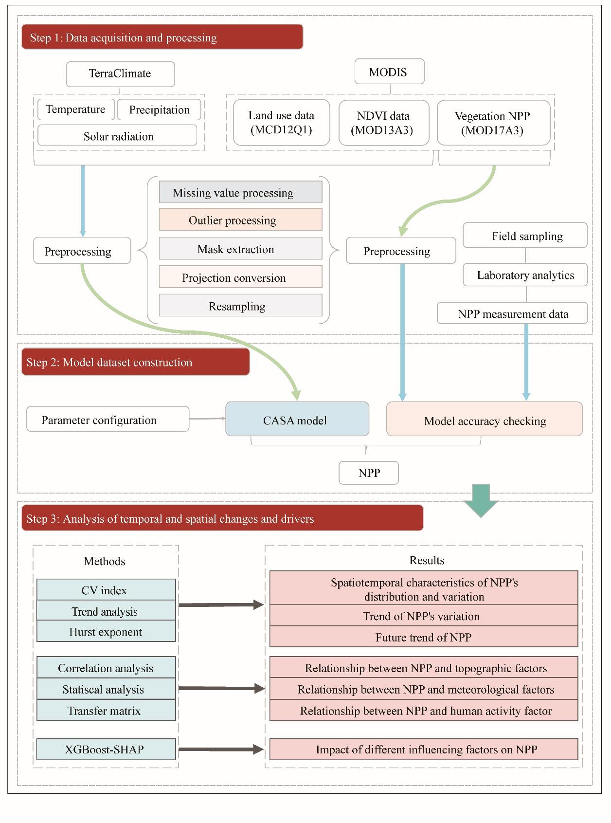
Fig. 2 Flowchart of the analytical workflow. MODIS, Moderate Resolution Imaging Spectroradiometer; NDVI, normalized difference vegetation index; NPP, net primary productivity; CASA, Carnegie-Ames-Stanford Approach; CV, coefficient of variation; XGBoost, Extreme Gradient Boosting; SHAP, SHapley Additive exPlanations.

3.1 NPP estimation using CASA model

This study estimated annual NPP during 2000-2020 at the pixel scale using CASA model, a remote-sensing light use efficiency model widely applied for regional and global NPP estimation (Zhou et al., 2025). Evaluations across diverse ecosystems indicated that CASA-based estimates showed good generality and stability (Zeng et al., 2024; Dong et al., 2025). In CASA, NPP was calculated as the product of absorbed photosynthetically active radiation (APAR) and actual light use efficiency (ε):
$\mathrm{NPP}_{(x, t)}=\operatorname{APAR}_{(x, t)} \times \mathcal{E}_{(x, t)}$,
$\operatorname{APAR}_{(x, t)}=\operatorname{SOL}_{(x, t)} \times \operatorname{FPAR}_{(x, t)} \times 0.5$,
$\mathcal{E}_{(x, t)}=\mathcal{E}_{\max } \times T_{\varepsilon 1(x, t)} \times T_{\varepsilon 2(x, t)} \times W_{\varepsilon(x, t)}$,
where NPP(x,t) is the NPP at pixel x in month t (g C/(m2•month)); APAR(x,t) is canopy absorbed photosynthetically active radiation (MJ/(m2•month)); ε(x,t) is the actual light use efficiency (g C/MJ); SOL(x,t) is total incoming shortwave solar radiation derived from the TerraClimate shortwave radiation product (MJ/(m2•month)); FPAR(x,t) is the fraction of absorbed photosynthetically active radiation; 0.5 represents the proportion of photosynthetically active radiation in total shortwave radiation; εmax is the maximum light use efficiency (g C/MJ) (Zhu et al., 2006); and Tε1(x,t), Tε2(x,t), and Wε(x,t) are the temperature- and moisture-stress scalars used to down-regulate εmax, with Tε1(x,t) and Tε2(x,t) accounting for temperature constraints via complementary response functions and Wε(x,t) representing water limitation (Zhu et al., 2007). The formulations of Tε1(x,t), Tε2(x,t), and Wε(x,t) have been applied and validated in arid and mountainous environments similar to the Tianshan Mountains (Liu et al., 2022; Heng and Wang, 2023; Zhang et al., 2024). Monthly NPP was summed to obtain annual NPP for each pixel for 2000-2020.
Field measurements were used to derive plot-based NPP estimates as independent references for evaluating CASA-derived NPP. A total of 265 vegetation sampling plots were established across the Tianshan Mountains in July 2018 and July 2024, stratified by elevation and ecosystem type (grassland and Picea schrenkiana Fisch. & C. A. Mey. forest). For grasslands, aboveground vegetation was harvested from 1 m by 1 m quadrats, oven-dried and plot-based grassland NPP was calculated as:
$\mathrm{NPP}_{g}=\mathrm{AGB} \times k$,
where NPPg is the plot-based annual grassland NPP (g C/(m2•a)); AGB is the aboveground dry biomass (g dry matter/m2); and k is the biomass-to-carbon conversion coefficient and was set to 0.45 in this study (Abdi et al., 2016; Wu et al., 2022).
For P. schrenkiana dominated forests, 10 m×10 m plots were established to quantify stand structure, including tree density, diameter at breast height, and tree height, and understory vegetation was surveyed in nested 1 m×1 m quadrats. Forest NPP was estimated as the sum of annual community growth and annual litter input (Wang et al., 2001).
$G=\frac{B}{\mathrm{c} T+\mathrm{d} B}$,
$L=\frac{1}{\frac{\mathrm{e}}{B}+\mathrm{f}}$,
$\mathrm{NPP}_{f}=G+L$,
where G is the annual community growth (kg C/(m2•a)); L is annual litter input (kg C/(m2•a)); NPPf is the annual forest NPP (kg C/(m2•a)); B is the stand biomass per unit area (kg dry matter/m2); T is the stand age (a); and c, d, e, and f are the forest-type constants. For spruce forests, c=0.4598, d=0.0069, e=10.1320, and f=0.0874 (Wang et al., 2009).
In MCD12Q1, "urban and built-up" was defined as pixels with at least 30.00% impervious surface and was termed "construction land" in this study. CASA-derived NPP over construction land therefore represented the productivity of vegetation within mixed pixels rather than impervious surfaces, which is essential for interpreting NPP patterns in urbanized areas.
To document uncertainty in key model inputs, we conducted consistency diagnostics for the meteorological forcing and land-cover information. Temperature and precipitation fields from TerraClimate and the NTPDC were compared in representative years (2000, 2005, 2010, 2015, and 2020) using correlation- and error-based metrics, and pixel-wise differences for 2020 were mapped. Land-cover products were also cross-compared for Built% and Crop%, and grids with absolute inter-product differences of at least 5.00% were identified as hotspots. To quantify the agreement between the TerraClimate and NTPDC datasets, we employed a suite of statistical metrics: the Pearson correlation coefficient and the Spearman's rank correlation coefficient to assess linear and monotonic relationships, respectively; the root mean square error (RMSE) and the median absolute error (MdAE) to measure the magnitude of average and typical deviations; and the mean bias error (MBE) to evaluate systematic over- or under-estimation. Detailed diagnostics are provided in the Supplementary Material (Tables S1 and S2; Figs. S1 and S2).
Table S1 Consistency of Built% and Crop% among land-cover products at the 6 km grid scale
Product pair Variable Spearman Pearson RMSE MdAE MBE Threshold Number of hotspots Share of grids (%)
IGBP vs. CLCD Built% 0.80* 0.78* 2.34 0.00 0.11 5 314 3.03
Crop% 0.77* 0.86* 10.98 0.00 0.01 5 1660 16.01
IGBP vs. LUCC Built% 0.83* 0.78* 3.72 0.00 0.76 5 505 4.87
Crop% 0.82* 0.83* 12.31 0.00 0.55 5 1909 18.41
CLCD vs. LUCC Built% 0.80* 0.74* 3.96 0.00 -0.64 5 611 5.89
Crop% 0.88* 0.96* 5.92 0.00 -0.54 5 1080 10.42

Notes: IGBP refers to the International Geosphere-Biosphere Programme (IGBP) land-cover classification scheme used by the MODIS land-cover product (MCD12Q1), LUCC refers to the Land Use and Cover Change (LUCC) dataset, and CLCD refers to the China Land Cover Dataset (CLCD). "Number of hotspots" is the count of 6 km grid cells whose absolute inter-product difference in Built% or Crop% is at least 5.00%. "Share of grids" is the percentage of all analyzed 6 km grid cells that satisfy the absolute difference ≥5.00%. RMSE, root mean square error; MdAE, median absolute error; MBE, mean bias error. MdAE values reported as 0.00 indicate that the median absolute difference is zero, meaning that at least half of the grid cells show identical Built% or Crop% between the compared products. *, significance at P<0.05 level.

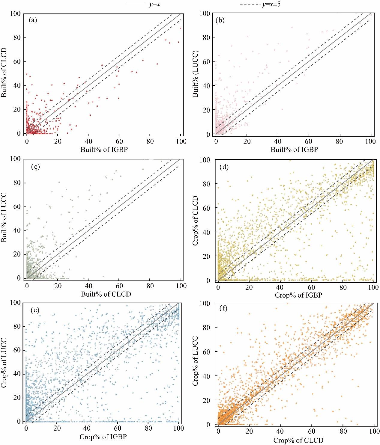
Fig. S1 Inter-product scatter plots of Built% and Crop% at the 6 km grid. The 1:1 line and ±5.00% bands are shown. (a), Built% compared between IGBP and CLCD; (b), Built% compared between IGBP and LUCC; (c), Built% compared between CLCD and LUCC; (d), Crop% compared between IGBP and CLCD; (e), Crop% compared between IGBP and LUCC; (f), Crop% compared between CLCD and LUCC. IGBP refers to the International Geosphere-Biosphere Programme (IGBP) land-cover classification scheme used by the MODIS land-cover product (MCD12Q1), LUCC refers to the Land Use and Cover Change (LUCC) dataset, and CLCD refers to the China Land Cover Dataset (CLCD).
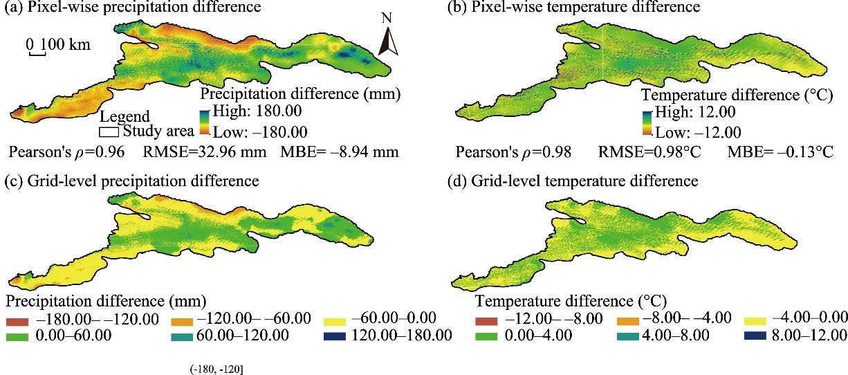
Fig. S2 Differences between the National Tibetan Plateau Data Center (NTPDC) temperature/precipitation (1 km) and TerraClimate temperature/precipitation (4 km resampled to 1 km) in 2020. (a), pixel-wise temperature difference; (b), pixel-wise precipitation difference; (c), grid-level temperature difference aggregated to the analysis grid; (d), grid-level precipitation difference aggregated to the analysis grid.

3.2 Quantification of NPP spatiotemporal metrics and trend slope statistics

Based on the pixel-level annual NPP product for 2000-2020, this study quantified spatiotemporal variability of NPP by integrating interannual dynamics, spatial patterns, stability, and trend significance. Interannual dynamics were summarized at the regional scale using total NPP and area-weighted mean NPP. Spatial patterns were characterized using multi-year mean NPP maps and zonal statistics across major land-cover types and environmental strata.
Interannual stability at the pixel level was quantified using the CV (Hou et al., 2015; Wei et al., 2022):
$\mathrm{CV}_{x}=\frac{\sigma_{x}}{\mathrm{NPP}_{x}}$,
where CVx is the coefficient of variation of annual NPP at pixel x; σx is the standard deviation of annual NPP at pixel x during 2000–2020 (g C/(m2•a)); and $ {\overline{\mathrm{NPP}_{x}}} $ is the corresponding multi-year mean annual NPP at pixel x (g C/(m2•a)). Long-term trends were estimated using the Theil–Sen median slope (Eastman et al., 2013; Tian et al., 2015):
$\text { Slope }_{x}=\operatorname{median}\left\{\frac{\mathrm{NPP}_{(x, j)}-\mathrm{NPP}_{(x, i)}}{j-i}\right\}_{1 \leq i<j \leq n}$,
where Slopex is the Theil-Sen slope of annual NPP at pixel x (g C/(m2•a)); NPP(x,i) and NPP(x,j) are the annual NPP values at pixel x in years i and j, respectively (g C/(m2•a)); and n is the number of years from 2000 to 2020, so here n=21.
Trend significance was evaluated using the Mann-Kendall test. The Mann-Kendall statistic Sx for pixel x was computed as (Hamed, 2008):
$S_{x}=\sum_{i=1}^{n-1} \sum_{j=i+1}^{n} \operatorname{sgn}\left(\mathrm{NPP}_{(x, j)}-\mathrm{NPP}_{(x, i)}\right)$,
$\operatorname{sgn}(\theta)=\left\{\begin{array}{ll} 1, & \theta>0 \\ 0, & \theta=0 \\ -1, & \theta<0 \end{array}\right.$.
When tied values occurred (i.e., two or more years had identical NPP values within the time series at a same pixel), the variance of Sx (Var(Sx)) was calculated with tie correction (Blain, 2013):
$\operatorname{Var}\left(S_{x}\right)=\frac{n(n-1)(2 n+5)-\sum_{k=1}^{g} t_{k}\left(t_{k}-1\right)\left(2 t_{k}+5\right)}{18}$,
where g is the number of tied groups; and tk is the size of the kth tied group.
The standardized test statistic Zx was then obtained as (Gocic and Trajkovic, 2013):
$Z_{x}=\left\{\begin{array}{ll} \frac{S_{x}-1}{\sqrt{\operatorname{Var}\left(S_{x}\right)}}, & S_{x}>0 \\ 0, & S_{x}=0 \\ \frac{S_{x}+1}{\sqrt{\operatorname{Var}\left(S_{x}\right)}}, & S_{x}<0 \end{array}\right.$.
The two-sided P-value (Px) was derived from Zx under the standard normal distribution (Sonali and Nagesh Kumar, 2013):
$P_{x}=2\left[1-\Phi\left(\left|Z_{x}\right|\right)\right]$,
where Ф is the cumulative distribution function of the standard normal distribution. Following the criteria summarized in Table 2, Px was used together with slopex to assign trend categories.
Table 2 Significance level and corresponding parameters for NPP trend
Significance level Slope P (two-sided)
Extremely significant reduction Slope<0.0000 P<0.01
Significant reduction Slope<0.0000 0.01≤P≤0.05
No significant change P>0.05
Significant increase Slope>0.0000 0.01≤P≤0.05
Extremely significant increase Slope>0.0000 P<0.01

3.3 Persistence and future trend analysis using the Hurst exponent

To assess the long-term persistence and future tendencies of NPP trends, we employed the Hurst exponent (H), a robust non-parametric method derived from rescaled range (R/S) analysis. The H value quantifies the autocorrelation or memory effect within a time series, indicating whether an observed trend is likely to persist, reverse, or behave randomly in the future (Bui and Ślepaczuk, 2022).
For a given annual NPP time series $\left\{N P P_{u}\right\}_{u=1}^{n}$ at a pixel (here n=21 for 2000–2020), the Hurst exponent (H) was estimated using the rescaled range (R/S) approach. For each segment length m (2≤mn; i.e., the number of annual observations in a subseries), the cumulative deviate series Xt,m was first computed as follows (Hamed, 2007):
$X_{t, m}=\sum_{u=1}^{t}\left(\mathrm{NPP}_{u}-\overline{\mathrm{NPP}}_{m}\right), \quad t=1,2, \ldots, m$,
$\overline{\mathrm{NPP}}_{m}=\frac{1}{m} \sum_{u=1}^{m} \mathrm{NPP}_{u}$,
where $\overline{\mathrm{NPP}}_{m}$ is the mean NPP of the same m-year subseries; u is the index in the summation; and t denotes the cumulative time step within the subseries. The range Rm and standard deviation Sm for each segment length m were then defined as (Mielniczuk and Wojdyłło, 2007):
$R_{m}=\max _{1 \leq t \leq m}\left(X_{t, m}\right)-\min _{1 \leq t \leq m}\left(X_{t, m}\right)$,
$S_{m}=\left[\frac{1}{m} \sum_{u=1}^{m}\left(\mathrm{NPP}_{u}-\overline{\mathrm{NPP}}_{m}\right)^{2}\right]^{1 / 2}$.
The rescaled range (R/S)m was calculated as (R/S)m=Rm/Sm. According to R/S theory, log(R/S)m exhibits a linear relationship with log(m) (Hamed, 2007):
$\log (R / S)_{m}=\mathrm{a}+H \log (m)$,
where a is the intercept. The Hurst exponent (H) was estimated as the slope of the ordinary least squares regression fitted to the log(m)-log(R/S)m relationship.
The Hurst exponent (H) indicates the persistence of a time series. Within an ecological context, this study established a comprehensive analytical framework: (1) determining whether the historical NPP trend represents degradation or improvement based on the direction of its slope; and (2) assessing the likely future trajectory by incorporating the persistence characteristics suggested by the H value. By integrating these two dimensions, 9 distinct categories describing future NPP dynamics are derived, as detailed in Table 3.
Table 3 Classification of future trends and corresponding parameters
Category Parameter Note
Strong persistent degradation (SPD) Slope< -0.0005 and 0.65<H<1.00 Strong historical decline with high persistence, likely to continue as severe degradation.
Weak persistent degradation (WPD) Slope< -0.0005 and 0.50<H<0.65 Moderate historical decline with moderate persistence, likely to continue as mild degradation.
Weak anti-persistent degradation (WAPD) Slope< -0.0005 and 0.35<H<0.50 Weak trend reversal with mild degradation, likely to reverse to weak degradation.
Strong anti-persistent degradation (SAPD) Slope< -0.0005 and 0.00<H<0.35 Strong trend reversal with significant degradation, likely to reverse to strong degradation.
Strong persistent improvement (SPI) Slope≥0.0005 and 0.00<H<0.35 Strong trend reversal with continuous improvement, likely to continue with significant improvement.
Weak anti-persistent improvement (WAPI) Slope≥0.0005 and 0.35<H<0.50 Weak trend reversal with mild improvement, likely to continue with weak improvement.
Moderate anti-persistent improvement (MAPI) Slope≥0.0005 and 0.50<H<0.65 Moderate trend reversal with improvement, likely to reverse to moderate improvement.
Strong anti-persistent improvement (SAPI) Slope≥0.0005 and 0.65<H<1.00 Strong trend reversal with significant improvement, likely to reverse to strong improvement.
No significant change (NSC) -0.0005<Slope<0.0005 Stable state with no significant trend, slight fluctuation.

3.4 Analysis of the driving mechanism

Fifteen variables capturing natural geography, climate, and anthropogenic pressure were used as drivers of NPP in this study. These include X1 (land use), X2 (temperature), X3 (precipitation), X4 (digital elevation model, DEM), X5 (slope), X6 (aspect), X7 (population density), X8 (GDP density),X9 (nighttime light index), X10 (human footprint), X11 (grazing intensity), X12 (distance to road), X13 (distance to highway), X14 (distance to water body), and X15 (distance to government center). These variables encompassed factors such as climate (temperature and precipitation), topography (elevation, slope, and aspect), human activities (population density, economic activity, grazing intensity, and accessibility), and land use. Using these variables, XGBoost modeled the nonlinear responses of NPP to multiple factors, and SHAP improved interpretability. XGBoost models complex nonlinear relationships by iteratively building an ensemble of decision trees, and its regularized objective reduces overfitting (Ma et al., 2025b). SHAP, grounded in Shapley values, attributes each variable's marginal contribution across feature combinations and quantifies both effect size and direction (Wu et al., 2024b):
$y=\phi_{0}+\sum_{k=1}^{M} \phi_{k}$,
where y is the model-predicted NPP for a given sample; ϕ0 is the expected (baseline) model output, i.e., the mean prediction of NPP; ϕk is the SHAP value representing the contribution of the kth feature to y; M is the number of input features (here M=15, corresponding to X1-X15).
Locally estimated scatterplot smoothing (LOESS) regression smoothed the SHAP dependency plots of major variables to explore their nonlinear responses and threshold effects on NPP. This method fits low-order polynomials to locally weighted samples without requiring predefined functions, effectively capturing variable trends and identifying critical intervals (Austin and Steyerberg, 2013). As a local fitting method, LOESS relies on data's local structure, necessitating a large and densely sampled dataset for stability and reliability. A 2 km×2 km grid with 90,348 cells was created in ArcGIS Pro to match the characteristics of LOESS fitting. NPP estimates and values of 15 drivers were assigned to each grid-cell center, enabling fine-scale analysis of driving mechanisms.

4 Results

4.1 Variation of land use from 2000 to 2020

Land-use change in the Tianshan Mountains from 2000 to 2020 was assessed with a seven-category transfer matrix, and land flows and transfer magnitudes were visualized (Fig. 3). From 2000 to 2010, grassland increased to 43.63% (+3.02%), mainly from unutilized land (14,295.99 km2), cropland (1871.76 km2), and wetland (1789.30 km2). Unutilized land decreased to 48.06%, mainly converting to grassland, cropland, and other ecological land. Cropland increased to 7.02%, with a net gain of 24.5% mainly from grassland. Wetland area shrank dramatically by 75.12% to 0.16% of the study area, with 1789.30 km2 converted to grassland, while forest area decreased by 45.65% to 0.28% of the study area. Meanwhile, water bodies decreased slightly from 0.48% to 0.43%, and construction land remained approximately 0.42%. From 2010 to 2020, ecological restoration and structural adjustment became evident. Forest rebounded by 20.20% and cropland expanded by 9.08%, largely at the expense of grassland (6739.33 km2). Grassland expansion (+2.34%) was driven primarily by conversion from unutilized land, which declined by 3.80% to 46.23%. Ecological recovery included wetland rebounding by 50.45% to 0.24% and water bodies increasing to 0.46%, while construction land remained near 0.42% with an increase of 0.84%. Overall, this period combined ecological recovery with cropland intensification.
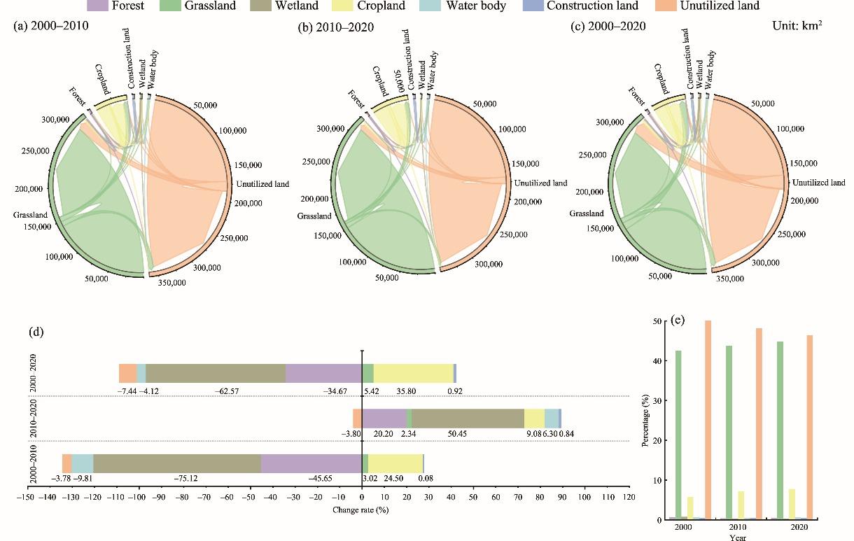
Fig. 3 Area (a-c), amplitude (d), and percentage (e) variations of different land use types in the Tianshan Mountains from 2000 to 2020
From 2000 to 2020, cropland increased to 7.65% (+35.80%), forest decreased to 0.34% (-34.67%), grassland reached 44.65%, and unutilized land declined to 46.23%. These changes informed the subsequent NPP analysis, as gains in grassland and cropland corresponded to higher NPP areas, whereas unutilized and degraded grasslands aligned with low-NPP zones. Percentages of construction land (Built%) and cropland (Crop%) were highly consistent among the land use products (MCD12Q1, LUCC, and CLCD), with points clustering along the 1:1 line and most deviations within ±5.00% (Fig. S1). Cross-product comparisons showed that Built% and Crop% were broadly consistent among land-cover datasets at the 6 km grid scale (Table S1), and most grid cells clustered around the 1:1 line within the ±5.00% band (Fig. S1). Nevertheless, 3.03%-18.41% of grids exceeded the ±5.00% threshold across product pairs (Table S1), indicating localized discrepancies in derived land-use proportions and thus spatially heterogeneous uncertainty.

4.2 Spatiotemporal variation of NPP from 2000 to 2020

4.2.1 Validation of the accuracy of CASA model estimation results

To validate the improved CASA model in the Tianshan Mountains, we made comprehensive comparisons with MODIS NPP and with field observations. The dataset comprised 265 sampling sites spanning ecological gradients and elevation zones in July 2018 and August 2024. The NPP estimates from the CASA model correlated strongly with both MODIS NPP (R2=0.704, P<0.01; Fig. 4a) and field measurements (R2=0.745, P<0.01; Fig. 4b).
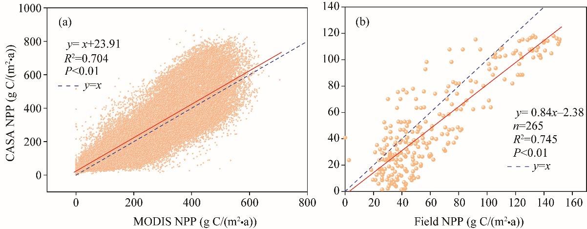
Fig. 4 Comparison of CASA NPP with MODIS NPP (a) and NPP of field sampling data (b)
Beyond validating against satellite products, the CASA framework offers key advantages for regional analysis. Its process-based design allows local parameter tuning and transparent uncertainty assessment, reducing dependence on any single remote-sensing product. Compatibility with 1 km driver datasets ensures spatial consistency for attribution analyses and supports temporal aggregation and scenario simulations. Meteorological validation corroborated dataset reliability, with multi-year 6 km correlations reaching ρ (both Pearson and Spearman coefficients)=0.99 for temperature and ρ=0.98 for precipitation (Table S2), and with 1 km cross-product agreement in 2020 providing additional support (Fig. S1).
Table S2 Year-specific consistency between TerraClimate and National Tibetan Plateau Data Center (NTPDC) meteorological datasets at the 6 km grid
Variable Year Pearson Spearman RMSE MdAE MBE
Temperature 2000 0.99 0.99 0.78 0.22 -0.10
2005 0.99 0.99 0.80 0.26 0.11
2010 0.99 0.99 0.80 0.25 -0.00
2015 0.99 0.99 0.83 0.23 0.15
2020 0.99 0.99 0.90 0.42 0.17
Precipitation 2000 0.98 0.99 22.74 8.07 -3.30
2005 0.98 0.98 24.69 9.00 -0.01
2010 0.98 0.98 30.01 10.68 -12.51
2015 0.98 0.98 30.05 12.60 -11.25
2020 0.96 0.96 33.57 20.89 9.49

4.2.2 Temporal characterization of NPP variation

From 2000 to 2020, total vegetation NPP in the Tianshan Mountains averaged 55.74 Tg C/a and ranged from 48.07 to 65.91 Tg C/a (Fig. 5a). Despite interannual fluctuations, NPP showed a slight upward trend (R2=0.053) with a steady rise from 2008 to 2011. NPP was lowest in 2014 at 48.07 Tg C and highest in 2016 at 65.91 Tg C, which exceeded the multi-year mean by 10.17 Tg C.
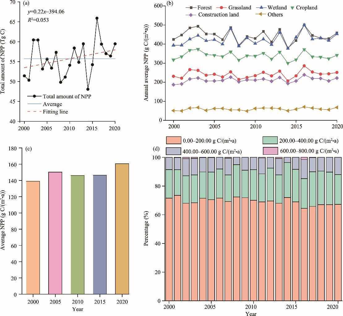
Fig. 5 Temporal variation of NPP in the Tianshan Mountains during 2000-2020. (a), total NPP; (b), annual mean NPP of different land use types; (c), average NPP in representative years; (d), area proportion of NPP classes. "Others" in Figure 5b include water body and unutilized land.
Most vegetation types showed generally increasing mean NPP trends from 2000 to 2020 (Fig. 5b). Forest consistently had the highest NPP, peaking at 500.62 g C/(m2•a) in 2016, closely followed by wetland at 499.59 g C/(m2•a). Cropland and grassland also increased, whereas construction land and unutilized land had the lowest mean NPP at 211.60 and 59.36 g C/(m2•a), respectively. NPP accounting included all land use types. Water body NPP comes mainly from phytoplankton and aquatic plants, offering a minor but comprehensive contribution to the regional carbon sink. Similarly, construction land NPP reflects vegetation within urban pixels (e.g., parks and gardens), representing carbon sequestration by urban green infrastructure. The NPP transfer matrix revealed substantial flows between land use types (Table 4). During 2000-2010, grassland and cropland gained the most NPP from unutilized land, with net transfers of 2.24×10¹² and 1.05×10¹² g C, respectively, making unutilized land the largest NPP source (-3.53×10¹² g C). From 2010 to 2020, grassland remained the primary net NPP beneficiary (+4.31×10¹² g C), mainly from unutilized land (+2.10×10¹² g C). Across both decades, grassland and cropland were the main NPP sinks, with unutilized land as the primary source.
Table 4 Transmission matrix of NPP variations between 2000 and 2020 (Unit: ×109 g C)
2000 2010
Construction land Cropland Forest Grassland Unutilized land Water body Wetland Transfer out
Construction land 35.20 35.20
Cropland -0.02 245.97 0.04 -186.35 -2.33 -5.17 0.21 52.33
Forest -0.13 23.65 -152.96 -16.14 0.20 -145.39
Grassland -0.01 783.67 11.54 23.81 -1382.36 -4.16 5.97 -561.54
Unutilized land 0.07 16.34 1.24 2849.02 655.97 0.51 3.00 3526.16
Water body 1.26 1.04 23.34 4.62 30.26
Wetland -0.21 1.73 -298.52 -11.53 -0.97 2.17 -307.34
Transfer in 35.23 1045.63 38.19 2236.27 -755.37 13.55 16.18 2629.68
2010 2020
Construction land Cropland Forest Grassland Unutilized land Water body Wetland Transfer out
Construction land 15.79 15.79
Cropland -0.54 -44.25 -402.79 -0.96 0.02 -448.52
Forest 26.60 -14.83 -3.87 0.96 8.86
Grassland -0.11 710.67 68.26 2632.71 -644.64 -1.35 77.50 2843.04
Unutilized land 52.21 1.40 2099.15 792.07 2.67 5.88 2953.38
Water body 2.20 -0.19 13.85 1.69 17.55
Wetland 1.39 -9.89 -1.15 -1.58 25.43 14.20
Transfer in 15.14 718.63 97.66 4306.54 141.27 13.59 111.48 5404.30

Note: Blank cells indicate values that around to 0.00, meaning that no detectable NPP transfer occurred for the corresponding land use transition.

Regional annual mean NPP rose from 138.97 to 160.69 g C/(m2•a) between 2000 and 2020, indicating sustained improvement in vegetation productivity (Fig. 5c). Spatially, over 90.00% of the area had annual mean NPP below 400.00 g C/(m2•a), dominated by 0.00-200.00 g C/(m2•a) at 64.49%-73.51%, followed by 200.00-400.00 g C/(m2•a) at 18.36%-24.34%. Higher productivity classes (≥400.00 g C/(m2•a)) were increasingly rare and together covered less than 10.00% of the area (Fig. 5d).

4.2.3 Spatial characterization of NPP variation

Spatial distribution (pixel-level mean) and interannual variability (CV) of NPP from 2000 to 2020 revealed pronounced heterogeneity. Mean NPP showed pronounced spatial heterogeneity (Fig. 6a). High NPP values clustered in the central and western northern slopes (e.g., Urumqi City, and Zhaosu County), characterized by higher elevations, forest/grassland dominance, and favorable hydrothermal conditions. Conversely, low NPP regions concentrated in the eastern and southern Tianshan Mountains (e.g., Hami Prefecture and Barkol Kazak Autonomous Region), featuring lower elevations, prevalent unutilized land, sparse vegetation, and constraints from aridity, soil salinization, and human disturbance. NPP CV ranged from 0.04 to 4.58, indicating substantial regional temporal variability (Fig. 6b). Ecosystems with low CV (high stability) showed minor interannual fluctuations, whereas high CV values (strong instability) concentrated in watersheds and unutilized lands, highlighting NPP sensitivity to climate variability and human disturbances.
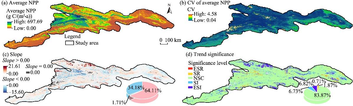
Fig. 6 Spatial patterns of NPP and its variability and trends in the Tianshan Mountains during 2000-2020. (a), multi-year mean NPP; (b), CV of annual NPP; (c), Theil-Sen trend slope of NPP; (d), significance level of NPP trends based on the Mann-Kendall test. ESR, extremely significant reduction; SR, significant reduction; NSC, no significant change; SI, significant increase; ESI, extremely significant increase. Inserted pie charts in Figure 6c and d show the area proportions of the corresponding categories.
NPP trends from 2000 to 2020 showed clear spatial heterogeneity, dominated by increasing trends (64.11%) against decreasing (34.18%) and near-zero trends (1.71%), indicating an overall upward trajectory (Fig. 6c). Slopes ranged from -15.60 to 21.61, with increases concentrated in forests and grasslands. Trend classification showed significant and extremely significant increase covering 6.73% and 6.82% of the area, concentrated in forest and grassland zones (Fig. 6d). By contrast, significant and extremely significant reduction covered 1.87% and 0.71% of the area and were scattered mainly in ecologically fragile unutilized lands and some wetlands. Despite overall growth, and most of the region showed no significant change at 83.88%, though localized degradation was evident.

4.3 Future trends of NPP in the Tianshan Mountains

Combining Hurst exponent (Fig. 7a) and slope (Fig. 6c), NPP trends in the Tianshan Mountains were classified into nine types, revealing marked spatial heterogeneity and distinct transition patterns (Table 4; Fig. 7b). NPP was projected to decline across much of the Tianshan Mountains, with SPD (36.41%) and WPD (17.52%) collectively covering 53.93% of the study area, primarily in central and northern areas, indicating a significant and spatially continuous degradation trend. WAPI at 13.63% and WAPD at 12.81% occurred mainly in central and western Tianshan Mountains, indicating reversals relative to historical trends with moderate dynamics. Improving trends were limited: SPI covered 4.97% and SAPI covered 0.36%, mainly in southern Tianshan Mountains, indicating low improvement potential. Regions classified as NSC covered 12.83%, were spatially scattered, and showed limited future variation. SAPD at 1.39% and MAPI at 0.07% comprised a very small share and were highly localized. Overall, persistent degradation was likely to dominate future NPP in the Tianshan Mountains, with localized and weak improvement and a strongly heterogeneous spatial pattern.
Fig. 7 Spatial distribution of the Hurst exponent (a) and projected future NPP trend types (b) in the Tianshan Mountains. SPD, strong persistent degradation; WPD, weak persistent degradation; WAPD, weak anti-persistent degradation; SAPD, strong anti-persistent degradation; SPI, strong persistent improvement; WAPI, weak anti-persistent improvement; MAPI, moderate anti-persistent improvement; SAPI, strong anti-persistent improvement; NSC, no significant change.

4.4 Nonlinear influence mechanisms of NPP

4.4.1 Contribution of impact factors to NPP

The XGBoost-SHAP method quantified the effects of 15 natural and human activity factors on vegetation NPP in the Tianshan Mountains (Fig. 8). Land use (X1) was the dominant factor (mean absolute SHAP value=29.54%), with low values (e.g., forest and grassland) promoting NPP and high values (e.g., construction land and unutilized land) suppressing it. Among climate factors, precipitation (X3, 16.03%) and temperature (X2, 11.05%) ranked second and third. Precipitation effects strengthened with higher values, whereas temperature effects were greater at lower values. DEM (X4), the most influential terrain factor (7.77%), had a positive effect at mid-altitudes but a strong negative effect at high altitudes. Among anthropogenic pressure factors, population density (X7, 8.10%) and GDP density (X8, 5.54%) had opposite effects. Population density shifted from negative to positive with increasing values, whereas high GDP density strongly suppressed NPP. Grazing intensity (X11, 6.06%) reduced NPP at high levels. Human footprint (X10, 3.88%) was mainly associated with negative effects at low values. Distance to road (X13, 4.27%) showed opposite effects at short and long distances. Nighttime light index (X9) and the remaining accessibility indicators (X12-X15) each contributed less than 3.00%.
Fig. 8 SHAP-based attribution of factors influencing NPP in the Tianshan Mountains. (a), SHAP summary (beeswarm) plot for the 15 predictors; (b), SHAP feature importance ranked by mean absolute SHAP values. X1, land use; X2, temperature; X3, precipitation; X4, DEM; X5, slope; X6, aspect; X7, population density; X8, gross domestic productivity (GDP) density; X9, nighttime light index; X10, human footprint; X11, grazing intensity; X12, distance to road; X13, distance to highway; X14, distance to water body; X15, distance to government center.
To reveal nonlinear responses and ecological thresholds of the top six drivers, we applied LOESS to SHAP dependence plots (Fig. 9). Land use (X1) showed a distinct nonlinear response: SHAP values peaked for wetland (near 150.00), followed by cropland and forest, indicating strong positive effects. Construction land and water body showed a dramatic shift to strongly negative values (near 100.00), while unutilized land had a marginally negative impact. For precipitation (X3), SHAP values turned positive near 250.00 mm and stabilized at 300.00-400.00 mm, indicating adequate water availability, with a slight decline above 400.00 mm suggesting diminishing returns or waterlogging stress. Temperature (X2) exhibited an inverted U-shape, with SHAP values rising sharply to a peak near 0.00°C before gradually declining, indicating saturation. A notable drop from 0.00°C to 10.00°C reflected heat and water stress, stabilizing at negative levels above 10.00°C. Population density (X7) showed a nonlinear response: SHAP values increased sharply to 500 people/km2, stabilized between 500-1500 people/km2 (positive saturation), and slightly declined above 1500 people/km2, suggesting increased ecological stress. For DEM (X4), SHAP values generally declined with altitude, despite a slight rebound at 1500-2000 m. A sharp drop above 3000 m highlighted severe suppression under high-altitude conditions. Grazing intensity (X11) showed a clear threshold response, with SHAP values peaking near 0.2 SU/hm2 (maximum benefit). Beyond this threshold, values declined rapidly and became strongly negative near -100 at intensities >8 SU/hm2, indicating a critical ecological limit.
Fig. 9 SHAP dependence plots showing nonlinear responses of NPP to the top six drivers in the Tianshan Mountains during 2000-2020. (a), land use (X1); (b), precipitation (X3); (c), temperature (X2); (d), population density (X7); (e), DEM (X4); (f), grazing intensity (X11). Points show SHAP values for each sample, and the red curve indicates the locally estimated scatterplot smoothing (LOESS)-smoothed trend.

4.4.2 Interactions between influence factors

SHAP interaction plots (Fig. 10) showed pairwise interactions among 15 factors affecting NPP in the Tianshan Mountains. Land use (X1) showed the strongest interactions, particularly with temperature (X2), precipitation (X3), and population density (X7), revealing distinct nonlinear patterns. The symmetric X1-X3 interaction indicated higher NPP potential for forest and cropland as precipitation increased, while the strong X1-X2 interaction showed that temperature effects on carbon sequestration depended strongly on land cover type. Precipitation (X3) interacted strongly with land use (X1) and with temperature (X2), population density (X7), and grazing intensity (X11), demonstrating compound regulation of NPP by hydrothermal conditions and anthropogenic pressure factors. In high-precipitation zones, the effects of population density and grazing intensity on NPP were altered or amplified. Temperature (X2) also interacted strongly with land use (X1), precipitation (X3), and the spatial factor distance to government center (X15), indicated that climate acted with spatial and anthropogenic influences to regulate NPP. For example, under high temperatures, well-developed areas showed divergent NPP responses, likely due to infrastructure advantages or distinct land use patterns. Interactions between population density (X7) and land use (X1) or climate were spatially clustered but high in magnitude, reinforcing the importance of human-nature coupling in shaping NPP. Although grazing density (X11) interacted less strongly with precipitation (X3) and population density (X7) than land use (X1) did, its nonlinear trends indicated that increased grazing pressure could alter precipitation's buffering effect on NPP. In contrast, interactions involving spatial variables were generally weak (SHAP values near zero), indicating largely independent and additive influences on NPP.
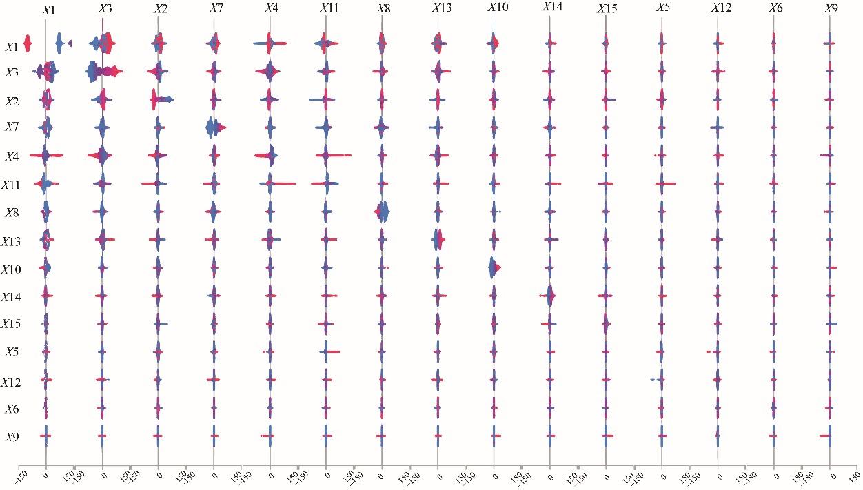
Fig. 10 Interaction plots of factors influencing NPP. The color gradient represents the feature values of the driving factors, of which red indicates high values, while blue represents low values.

4.5 Integrated diagnostics of future risk and driving mechanisms

Integrated diagnostics confirmed that persistent degradation would affect over half of the region, concentrated in specific transition zones. This trend was primarily driven by the dominant role of land use, coupled with critical hydroclimatic thresholds and amplifying anthropogenic pressures. Complex nonlinear interactions among these drivers further intensified the degradation risks in identified hotspots. At the 6 km scale, we cross-validated two consistent four-class disturbance schemes with an identical type definition (I-IV; Table S3): the human disturbance four-type hydrothermal-regime clustering (HD4) and an independent rule-based disturbance classification. HD4 delineates the four types via clustering based on hydrothermal conditions and human-pressure proxies (Built%, Crop%, grazing intensity, population density, and GDP), whereas the rule-based scheme assigns the same four types using predefined thresholds of these indicators. The two schemes showed strong agreement (overall accuracy=83.79% and Kappa coefficient=0.71; Table S3). Most mismatches were mainly concentrated in mixed transition cells between types II and III and between types I and IV (Fig. S3).
Table S3 Confusion matrix between human disturbance four-type hydrothermal-regime clustering (HD4) and the rule-based classification (6 km grids; n=10,368)
Human disturbance type Rule-based classification Producer's Accuracy (%)
5297 0 30 67 98.20
70 79 40 26 36.70
429 25 684 81 56.10
835 0 77 2628 74.30
User's accuracy (%) 79.80 76.00 82.30 93.80
Overall accuracy=83.79% Expected agreement=0.43 Kappa coefficient=0.71

Note: I corresponds to grids dominated by high-altitude or desert landscapes with minimal human impact; II represents urban-industrial settings characterized by high imperviousness and elevated population density and GDP; III denotes agricultural-irrigated grids dominated by cropland and irrigation; and IV corresponds to pastoral-grazing settings where grassland use and grazing pressure are prevalent. The HD4 and the rule-based scheme adopt an identical four-type definition; therefore, the confusion matrix compares the same disturbance categories derived from two independent procedures.

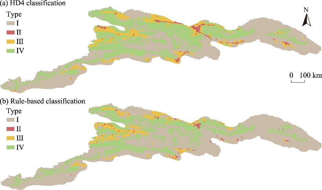
Fig. S3 Spatial distribution of human disturbance four-type hydrothermal-regime clustering (HD4; a) and rule-based classification in 2020. I corresponds to grids dominated by high-altitude or desert landscapes with minimal human impact; II represents urban-industrial settings characterized by high imperviousness and elevated population density and GDP; III denotes agricultural-irrigated grids dominated by cropland and irrigation; and IV corresponds to pastoral-grazing settings where grassland use and grazing pressure are prevalent. The HD4 derives the four types via clustering based on hydrothermal conditions and human-pressure proxies, whereas the rule-based scheme assigns the same types using predefined thresholds of Built%, Crop%, grazing intensity, population density, and GDP.
The 2024 diagnostics revealed synergy hotspots along oasis-desert ecotones and urban fringes. Threshold screening identified high-risk grids covering 3.88% of the study area (Fig. S4), with widespread low NPP values along arid margins. Across all 2 km grid cells in the study area, the 2024 mean values were 202.31 g C/(m2•a) for NPP, 269.05 mm for precipitation, 3.53°C for temperature, 0.51% for Built%, and 6.51% for Crop%. The spatial pattern aligned with SHAP-based thresholds, indicating that hydrothermal stress combined with anthropogenic pressure governs near-term NPP risk.
Fig. S4 Near-term ecosystem productivity risk in the Tianshan Mountains in 2024 at the 2 km grid. (a), synergy hotspot; (b), high-risk grid distribution; (c), NPP low tail. Synergy hotspots are grids with NPP in the lowest 30.00% of all 2 km grids, together with hydroclimatic stress (precipitation in the lowest 40.00% or temperature in the highest 40.00%) and elevated human pressure (population density in the highest 30.00% or a built-up proportion of at least 10.00%). High-risk grids are synergy hotspots where hydroclimatic conditions further deviate from the identified safe ranges. Specifically, precipitation falls below 300.00 mm or exceeds 400.00 mm, or temperature falls below -5.00°C or exceeds 5.00°C. NPP low tail includes grids with NPP in the lowest 30.00% only, regardless of hydroclimatic or human-pressure conditions. The 30.00%, 40.00%, and 30.00% thresholds are percentile-based cutoffs computed across all 2 km grids, whereas the 10.00% built-up cutoff is an absolute threshold.

5 Discussion

5.1 Response of NPP to land use change

NPP, a key indicator of terrestrial carbon cycling, is highly sensitive to land use change, reflecting the combined effects of human and natural processes on ecosystem structure and function (Zeng et al., 2025). In the Tianshan Mountains, the overall NPP increase from 2000 to 2020 was closely linked to land use changes, primarily driven by grassland and cropland expansion under favorable mid- to low-elevation hydrothermal conditions (Liu et al., 2021). This expansion enhanced regional carbon fixation through higher photosynthetic efficiency and biomass accumulation. This pattern aligned with Hou (2020), who reported that cropland and grassland expansion dominated NPP increase in the Weigan-Kuqa River Basin, Xinjiang Uygur Autonomous Region, China. Converting unutilized land to ecological types like grassland optimizes ecological space, enhancing soil-water conservation and carbon sequestration (Hu et al., 2025). This positive link between intensive land management and enhanced ecosystem services is common in arid western China (Guo and Zhang, 2021).
Despite localized recovery under return-to-forest programs, forest did not offset prior degradation. Due to limited forest area and slow growth rates, forest's short-term contribution remained constrained (Pang et al., 2024). Similarly, wetland exhibited high per-area NPP due to moisture availability and national greening efforts, despite their limited spatial extent. However, both forests and wetlands experienced net declines over the study period, weakening their overall regional NPP support (Xiang et al., 2023; Ren et al., 2025). Construction land expanded slowly but reduced NPP through surface sealing and heat-island effects, especially along urban fringes (Niu et al., 2024). Note that NPP for construction land does not originate from impervious surfaces, but reflects the productivity of vegetation components (e.g., urban parks, lawns, and street trees) within these mixed pixels, as defined by our land cover classification (Liu et al., 2024). Consequently, land use management should prioritize optimizing ecological space and protecting high-value ecosystems to sustain productivity and carbon sequestration.

5.2 Analysis of NPP influences on vegetation in the Tianshan Mountains

NPP in the Tianshan Mountains resulted from a complex coupling of human activity, land use, and climate. Among these factors, land use type explained the largest share of NPP variability. Ecological lands enhanced NPP by increasing vegetation cover and improving local conditions, while construction land reduces it through surface sealing and habitat fragmentation. The SHAP analysis correctly captured this suppressive effect. However, the non-zero NPP value assigned to construction land underscored that our model estimates reflect the productivity of the integrated pixel (Luo and Wang, 2009). This interpretation aligns with the land cover definition and highlights that the CASA model, while powerful, attributes productivity to the entire mixed pixel rather than isolating the null contribution of impervious surfaces. Unutilized land currently had low productivity due to poor soils but held significant potential for ecological restoration, aligning with evidence that ecological lands promote productivity whereas non-ecological lands constrain it (Li et al., 2023). The pattern of wetland NPP exceeding that of grassland in the Tianshan Mountains, driven by stable water supply alleviating moisture stress, underscored the primary control of precipitation (Chen et al., 2023). This key climatic driver exhibited an optimal window of 300.00-400.00 mm, alongside a temperature threshold near 0.00°C, which collectively confirmed the strong hydrothermal regulation in arid areas (Huxman et al., 2004). Anthropogenic pressures were nonlinear. Moderate population and GDP density promoted NPP, whereas high-density development imposed stress and reduced productivity. Grazing showed low-intensity promotion and high-intensity suppression, indicating grassland sensitivity and the benefits of moderate grazing (Suo et al., 2023). These controls aligned with national and regional evidence on climate and human effects (Wei et al., 2025). At the 6 km scale, robustness tests showed strong agreement between the human disturbance hydrothermal-regime clustering and the rule-based scheme. Consistent with the SHAP-based attribution, land use and hydroclimatic conditions dominated NPP variability, while anthropogenic pressure acted as an important modifier in hotspot areas.
Near-term diagnostics for 2024 linked mechanisms to management (Fig. S4). High-risk grids clustered along these belts, accounting for 3.88% of the study area effectively evaluated region. Priority actions should include water-saving irrigation and allocation, grazing control or rotation, and peri-urban greening and ecological corridors. The spatial concordance between high-risk areas and projected persistent-degradation zones supported using the identified thresholds and interaction mechanisms for early warning and targeted intervention. Unlike plain-type arid areas (e.g., Ningxia Hui Autonomous Region), degradation in the Tianshan Mountains clusters along ecotones and peri-urban fringes under orographic amplification (Cong et al., 2025). This reflected the co-occurrence of water or heat stress with anthropogenic pressure, consistent with known vegetation-specific drought responses and the dominant role of topography and climate in mountain basins (Wu et al., 2024a; Zhang et al., 2025).

5.3 Limitations and prospects

CASA performed well in the Tianshan Mountains, consistent with Pan and Li (2015), who reported a high correlation (R2=0.870) for an improved version in the Northwest China. However, model-level uncertainties remain. In extremely arid zones, CASA can be biased due to the simplified moisture stress term (Bao et al., 2016). Transferring the εmax parameter across regions may introduce magnitude uncertainty, necessitating future calibration for the Tianshan Mountains using site-level flux and plot data (Guan et al., 2022). CASA also tends to underestimate NPP compared with MODIS products and field measurements. Potential reasons include uncertainties in validation data (e.g., sampling bias toward high-productivity sites), the limited ability of MOD17A3 to capture vegetation-soil-moisture heterogeneity, and spatiotemporal scale mismatches (Wen et al., 2022; Wang et al., 2023).
Since MODIS and CASA both rely on remote sensing and meteorological drivers, they are not fully independent. Our dual validation provides convergent evidence but does not eliminate dependence. At the data level, the main analyses employ TerraClimate data resampled from 4 km to 1 km, a process that may attenuate fine-scale climatic signals. A scale check against higher-resolution NTPDC data at 1 km and 6 km scales showed close agreement with small deviations, indicating limited scale-related uncertainty for analysis. Cross-product validation at the 6 km scale confirmed high overall consistency. In contrast, a 1 km analysis revealed localized discrepancies, particularly within ecological transition zones. The anthropogenic footprint data lacked explicit disturbance types, which constrained the diagnosis of underlying mechanisms (Ellis, 2011). The 500 m resolution of MCD12Q1 limited the detection of fine-scale land use changes and exacerbated class mixing in urban-oasis transition zones. This led to overestimated NPP for construction land, causing local overestimation or underestimation and regional aggregation errors (Huang et al., 2021; Wu et al., 2023). Because wetland-water boundaries and seasonal inundation can blur at 500 m, local overestimation of wetland NPP is possible.
Future research should incorporate advanced moisture stress algorithms to improve accuracy in arid areas and calibrate the εmax parameter locally using tower flux and plot-level data. To achieve a more accurate attribution of NPP dynamics, future work must incorporate high-resolution data on climate, land use, and explicit anthropogenic disturbance types, including grazing intensity and infrastructure development, to overcome scale-related biases. We can further integrate multi-source data, such as unmanned aerial vehicle (UAV) remote sensing and satellite-derived soil moisture, across scales to reconcile model discrepancies and reduce uncertainties, enabling more reliable assessments of ecosystem productivity in vulnerable transition zones.

6 Conclusions

Using an integrated CASA-Hurst-XGBoost framework, this study quantified spatiotemporal NPP dynamics across the Tianshan Mountains and attributed their controls to coupled hydroclimatic constraints and anthropogenic pressure. The results demonstrated that NPP trajectories are governed by hydrothermal thresholds together with anthropogenic pressure, and that degradation tends to occur where these drivers interact synergistically.
Across the study area, recent NPP gains were closely associated with land use optimization, particularly the expansion of grassland and cropland and the decline of unutilized land. Notably, grassland expansion generated a substantial carbon sink of 4.31×10¹² g C during 2010-2020, underscoring the carbon-management value of grassland conservation and well-guided land conversion. Despite an overall increase in NPP, the system exhibited pronounced spatial heterogeneity: productivity was higher in central-western regions and northern slopes (e.g., Urumqi City and Zhaosu County) but lower along arid margins such as Hami Prefecture. Meanwhile, persistent degradation dominated 53.93% of the landscape, whereas strong improvement accounted for only 4.97%, a pattern shaped by hydroclimatic gradients that signaled low resilience—especially in ecotones—and highlighted the urgency of prioritized restoration and zoned management to avert irreversible losses.
Model interpretation further indicated that nonlinear thresholds and interactions dominate the NPP response. Land use type emerged as the strongest predictor, and critical hydrothermal thresholds were identified at 300.00-400.00 mm precipitation and near 0.00°C temperature, beyond which productivity declined sharply. Population and GDP density as well as grazing intensity exerted nonlinear effects—enhancing NPP at low levels but suppressing NPP at high levels—and their nonlinear coupling concentrated persistent degradation hotspots along oasis-desert ecotones and urban fringes. Collectively, these findings condensed to a central conclusion: sustaining and enhancing NPP in arid mountain systems requires simultaneously respecting hydrothermal thresholds and managing anthropogenic pressure, particularly where their interactions amplify degradation risk.
This work provides a threshold-based decision framework for arid mountain ecosystem management. We recommend targeted interventions in vulnerable oasis-desert ecotones and peri-urban zones, including water-saving irrigation, grazing rotation, and the construction of ecological corridors, to mitigate compounded risks from climate change and anthropogenic pressure. Future research should incorporate higher-resolution climate and land datasets to improve predictive accuracy and strengthen decision support.

Conflict of interest

The authors declare that they have no known competing financial interests or personal relationships that could have appeared to influence the work reported in this paper.

Acknowledgements

This research was supported by the Natural Science Foundation of Xinjiang Uygur Autonomous Region (2023E01006, 2024TSYCCX0004).

Author contributions

Conceptualization: XU Zhonglin, YANG Jianjun; Data curation: LI Jiani, WANG Yao; Methodology: LI Jiani, XU Denghui, XU Zhonglin, YANG Jianjun; Investigation: LI Jiani, WANG Yao; Formal analysis: XU Denghui, XU Zhonglin, YANG Jianjun; Writing - original draft preparation: LI Jiani, XU Denghui; Writing - review and editing: LI Jiani, WANG Yao; Funding acquisition: XU Zhonglin, WANG Yao; Resources: YANG Jianjun; Supervision: WANG Yao, XU Zhonglin; Project administration: WANG Yao; Software: LI Jiani, XU Denghui; Validation: LI Jiani, XU Denghui, XU Zhonglin; Visualization: XU Denghui, YANG Jianjun. All authors approved the manuscript.
[1]
Abdi A M, Vrieling A, Yengoh G T, et al. 2016. The El Niño - La Niña cycle and recent trends in supply and demand of net primary productivity in African drylands. Climatic Change, 138(1): 111-125.

DOI

[2]
Ahlström A, Raupach M R, Schurgers G, et al. 2015. The dominant role of semi-arid ecosystems in the trend and variability of the land CO₂ sink. Science, 348(6237): 895-899.

DOI PMID

[3]
Austin P C, Steyerberg E W. 2013. Graphical assessment of internal and external calibration of logistic regression models by using loess smoothers. Statistics in Medicine, 33(3): 517-535.

[4]
Bao G, Bao Y H, Qin Z H, et al. 2016. Modeling net primary productivity of terrestrial ecosystems in the semi-arid climate of the Mongolian Plateau using LSWI-based CASA ecosystem model. International Journal of Applied Earth Observation and Geoinformation, 46: 84-93.

DOI

[5]
Blain G C. 2013. The modified Mann-Kendall test: on the performance of three variance correction approaches. Bragantia, 72(4): 416-425.

DOI

[6]
Bui Q, Ślepaczuk R. 2022. Applying Hurst exponent in pair trading strategies on Nasdaq 100 index. Physica A: Statistical Mechanics and its Applications, 592: 126784, doi: 10.1016/j.physa.2021.126784.

[7]
Chen S, Zhao W W, Han Y. 2023. Spatio-temporal variation of vegetation precipitation use efficiency in arid and semi-arid regions of China. Acta Ecologica Sinica, 43(24): 10295-10307. (in Chinese)

[8]
Chen T Q, Guestrin C. 2016. XGBoost: a scalable tree boosting system. In: KDD '16: Proceedings of the 22nd ACM SIGKDD International Conference on Knowledge Discovery and Data Mining. Association for Computing Machinery's Special Interest Group on Knowledge Discovery and Data Mining (ACM SIGKDD). San Francisco, USA, 785-794.

[9]
Chen W D, Liu X H, Li H Y, et al. 2024a. Ecosystem service function and security pattern of Tianshan Mountains in Xinjiang from 1990 to 2050. Geology in China, 51(5): 1644-1663. (in Chinese)

[10]
Chen Y N, Li W H, Deng H J, et al. 2016. Correction: Corrigendum: Changes in Central Asia's water tower: past, present and future. Scientific Reports, 6: 39364, doi: 10.1038/srep39364.

PMID

[11]
Chen Y N, Fang G H, Li Z, et al. 2024b. The crisis in oases: research on ecological security and sustainable development in arid regions. Annual Review of Environment and Resources, 49: 1-20.

DOI

[12]
Cong S X, Ding X D, Chang W J, et al. 2025. Response of net primary productivity to drought change in middle arid zone of Ningxia Hui Autonomous Region. Bulletin of Soil and Water Conservation, 45(4): 402-412. (in Chinese)

[13]
Dong D J, Zhang R H, Guo W, et al. 2025. Assessing spatiotemporal dynamics of net primary productivity in Shandong Province, China (2001-2020) using the CASA model and Google Earth Engine: trends, patterns, and driving factors. Remote Sensing, 17(3): 488, doi: 10.3390/rs17030488.

[14]
Du Y J, Li X L, He X L, et al. 2025. Spatiotemporal variation characteristics and driving mechanisms of net primary productivity of vegetation on northern slope of Tianshan Mountains based on CASA model, China. Plants (Basel), 14(16): 2499, doi: 10.3390/plants14162499.

[15]
Eastman J R, Sangermano F, Machado E A, et al. 2013. Global trends in seasonality of normalized difference vegetation index (NDVI), 1982-2011. Remote Sensing, 5(10): 4799-4818.

DOI

[16]
Ellis E C. 2011. Anthropogenic transformation of the terrestrial biosphere. Philosophical Transactions of the Royal Society A: Mathematical, Physical, and Engineering Sciences, 369: 1010-1035.

[17]
Friedlingstein P, O'Sullivan M, Jones M W, et al. 2023. Global carbon budget 2023. Earth System Science Data, 15(12): 5301-5369.

DOI

[18]
Gocic M, Trajkovic S. 2013. Analysis of changes in meteorological variables using Mann-Kendall and Sen's slope estimator statistical tests in Serbia. Global and Planetary Change, 100: 172-182.

DOI

[19]
Grekousis G. 2025. Geographical-XGBoost: a new ensemble model for spatially local regression based on gradient-boosted trees. Journal of Geographical Systems, 27(2): 169-195.

DOI

[20]
Guan X B, Chen J M, Shen H F, et al. 2022. Comparison of big-leaf and two-leaf light use efficiency models for GPP simulation after considering a radiation scalar. Agricultural and Forest Meteorology, 313: 108761, doi: 10.1016/j.agrformet.2021.108761.

[21]
Guo Z P, Zhang X D. 2021. Differentiated Land Policy and the Coordination Logic to Spatial Elements—Taking "One Decrease Three Increase" of Un-Utilized Land in Lanzhou for Example. Construction & Design for Engineering, 12: 177-179, 183. (in Chinese)

[22]
Hamed K H. 2007. Improved finite-sample Hurst exponent estimates using rescaled range analysis. Water Resources Research, 43(4): W04413, doi: 10.1029/2006WR005111.

[23]
Hamed K H. 2008. Trend detection in hydrologic data: The Mann-Kendall trend test under the scaling hypothesis. Journal of Hydrology, 349(3-4): 350-363.

DOI

[24]
Heng R, Wang X J. 2023. NPP prediction of vegetation in Gurbantunggut Desert based on CASA model. Water Resources and Hydropower Engineering, 54(12): 189-201. (in Chinese)

[25]
Hou W J, Gao J B, Wu S H, et al. 2015. Interannual variations in growing-season NDVI and its correlation with climate variables in the southwestern karst region of China. Remote Sensing, 7(9): 11105-11124.

DOI

[26]
Hou Y F. 2020. Impacts of land use/cover change on vegetation net primary productivity in the Weigan-Kuqa River Basin, Xinjiang. MSc Thesis. Urumqi: Xinjiang Agricultural University. (in Chinese)

[27]
Hu J H, Song M F, Zhang L W. 2025. Spatial and temporal evolution of land use carbon emission and carbon balance zoning: evidence from Xinjiang China. Scientific Reports, 15: 35705, doi: 10.1038/s41598-025-19475-9.

[28]
Huang J, Huang H S, Zhong H Y, et al. 2021. Provincial-scale applicability analysis of land cover data at different resolutions—case study of Jiangxi Province. Jiangxi Science, 39(3): 534-540, 551. (in Chinese)

[29]
Huang J P, Yu H P, Guan X D, et al. 2016. Accelerated dryland expansion under climate change. Nature Climate Change, 6: 166-171.

DOI

[30]
Huxman T E, Smith M D, Fay P A, et al. 2004. Convergence across biomes to a common rain-use efficiency. Nature, 429: 651-654.

DOI

[31]
IPCC Intergovernmental Panel on Climate Change. 2021. Climate Change 2021: The Physical Science Basis. Contribution of Working Group I to the Sixth Assessment Report of the Intergovernmental Panel on Climate Change. Cambridge and New York: Cambridge University Press, 2391.

[32]
Jiang F G, Deng M L, Long Y, et al. 2022. Spatial pattern and dynamic change of vegetation greenness from 2001 to 2020 in Tibet, China. Frontiers in Plant Science, 13: 892625, doi: 10.3389/fpls.2022.892625.

[33]
Kalisa W, Igbawua T, Henchiri M, et al. 2019. Assessment of climate impact on vegetation dynamics over East Africa from 1982 to 2015. Scientific Reports, 9: 16865, doi: 10.1038/s41598-019-53150-0.

PMID

[34]
Li Q, Yang T, Zhou H F, et al. 2019. Patterns in snow depth maximum and snow cover days during 1961-2015 period in the Tianshan Mountains, Central Asia. Atmospheric Research, 228: 14-22.

DOI

[35]
Li Y, Shang R, Qu Y B, et al. 2023. Assessment of the dynamics of vegetation net primary productivity and its response to environmental chan-ges before and after the Grain for Green Project: A case study from the Loess Plateau of Northern Shaanxi. Water Resources and Hydropower Engineering, 54(06): 156-166, doi: 10.13928/j.cnki.wrahe.2023.06.014. (in Chinese)

[36]
Liang L, Li M, Huang Z R, et al. 2025. Insights into spatiotemporal dynamics and driving mechanisms of vegetation net primary productivity in African terrestrial ecosystems. International Journal of Applied Earth Observation and Geoinformation, 143: 104824, doi: 10.1016/j.jag.2025.104824.

[37]
Liu L, Guan J Y, Mu C, et al. 2022. Spatio-temporal characteristics of vegetation net primary productivity in the Ili River Basin from 2008 to 2018. Acta Ecologica Sinica, 42(12): 4861-4871. (in Chinese)

[38]
Liu Y D, Yao X J, Li Z S, et al. 2024. Impacts of climate change and land use/cover change on the net primary productivity of vegetation in Hexi Region, Northwest China. Arid Zone Research, 41(1): 169-180. (in Chinese)

DOI

[39]
Liu Z J, Liu Y S, Wang J Y. 2021. A global analysis of agricultural productivity and water resource consumption changes over cropland expansion regions. Agriculture, Ecosystems & Environment, 321: 107630, doi: 10.1016/j.agee.2021.107630.

[40]
Lu Y Y, Xu X L, Li J C, et al. 2022. Research on the spatio-temporal variation of carbon storage in the Xinjiang Tianshan Mountains based on the InVEST model. Arid Zone Research, 39(6): 1896-1906. (in Chinese)

DOI

[41]
Lundberg S M, Lee S I. 2017. A unified approach to interpreting model predictions. In: von Luxburg U, Guyon I. NIPS'17: Proceedings of the 31st International Conference on Neural Information Processing Systems (NIPS). NIPS. Long Beach, USA. 4768-4777.

[42]
Luo Y, Wang C L. 2009. Valuation of the net primary production of terrestrial ecosystems in Guangdong Province based on remote sensing. Ecology and Environmental Sciences, 18(4): 1467-1471. (in Chinese)

[43]
Ma R L, Xue Y Y, Chen J L, et al. 2025a. Tradeoffs and synergies in carbon-water coupling of vegetation across China's arid and semiarid regions. Arid Zone Research, http://link.cnki.net/urlid/65.1095.X.20251126.1421.008. (in Chinese)

[44]
Ma Z L, Han M, Kong X L, et al. 2025b. Interpretability-driven analysis of carbon storage in the Yellow River Delta based on SHAP-XGBoost model. Environmental Science, doi: 10.13227/j.hjkx.202505105. (in Chinese)

[45]
Mielniczuk J, Wojdyłło P. 2007. Estimation of Hurst exponent revisited. Computational Statistics & Data Analysis, 51(9): 4510-4525.

[46]
Niu J Q, Wang Z Y, Lin H, et al. 2024. Temporal and spatial evolution characteristics and driving factors of NPP in the Huaihe River Economic Belt. Geography and Geo-Information Science, 40(3): 37-43. (in Chinese)

[47]
Pang W L, Ji P H, Pang L D, et al. 2024. Spatial and temporal evolution of land use pattern and ecosystem service function in Daxinganling Mountains of Inner Mongolia. Bulletin of Soil and Water Conservation, 44(4): 340-351, 361. (in Chinese)

[48]
Ren Y X, Mao D H, Wang T, et al. 2025. Persistent vegetation greening trends across China's wetlands. Communications Earth & Environment, 6: 624, doi: 10.1038/s43247-025-02628-z.

[49]
Robinson N P, Allred B W, Smith W K, et al. 2018. Terrestrial primary production for the conterminous United States derived from Landsat 30 m and MODIS 250 m. Remote Sensing in Ecology and Conservation, 4(3): 264-280.

DOI

[50]
Suo C X, Fei X, Liu Y Z, et al. 2023. Functional group characteristics of plant community at different grazing intensities in alpine grassland of northwestern Sichuan. Chinese Journal of Applied and Environmental Biology, 29(1): 109-116. (in Chinese)

[51]
Sonali P, Nagesh Kumar D. 2013. Review of trend detection methods and their application to detect temperature changes in India. Journal of Hydrology, 476: 212-227.

DOI

[52]
Tian F, Fensholt R, Verbesselt J, et al. 2015. Evaluating temporal consistency of long-term global NDVI datasets for trend analysis. Remote Sensing of Environment, 163: 326-340.

DOI

[53]
Turner D P, Ritts W D, Cohen W B, et al. 2006. Evaluation of MODIS NPP and GPP products across multiple biomes. Remote Sensing of Environment, 102(3-4): 282-292.

DOI

[54]
Wang B, Liu M C, Zhang B. 2009. Dynamics of net production of Chinese forest vegetation based on forest inventory data. Forest and Grassland Resources Research, 1: 35-43. (in Chinese)

[55]
Wang S J, Zhang M J, Hughes C E, et al. 2016. Factors controlling stable isotope composition of precipitation in arid conditions: an observation network in the Tianshan Mountains, Central Asia. Tellus Series B: Chemical and Physical Meteorology, 68(1): 26206, doi: 10.3402/tellusb.v68.26206.

[56]
Wang T, Bao A M, Xu W Q, et al. 2023. Dynamics of forest net primary productivity based on tree ring reconstruction in the Tianshan Mountains. Ecological Indicators, 146: 109713, doi: 10.1016/j.ecolind.2022.109713.

[57]
Wang Y H, Zhou G S, Jiang Y L, et al. 2001. Estimating biomass and NPP of Larix forests using forest inventory data (FID). Acta Phytoecologica Sinica, 25(4): 420-425. (in Chinese)

[58]
Wei Q, Zhou B R, Wang W Y. 2025. Qinghai Province (Tibetan Plateau): quantifying the influence of climate change and human activities on vegetation net primary productivity and livestock carrying capacity growth potential. Biology, 14(5): 494, doi: 10.3390/biology14050494.

[59]
Wei X D, Yang J, Luo P P, et al. 2022. Assessment of the variation and influencing factors of vegetation NPP and carbon sink capacity under different natural conditions. Ecological Indicators, 138: 108834, doi: 10.1016/j.ecolind.2022.108834.

[60]
Wen J G, Wu X D, Wang J P, et al. 2022. Characterizing the effect of spatial heterogeneity and the deployment of sampled plots on the uncertainty of ground "truth" on a coarse grid scale: case study for near-infrared (NIR) surface reflectance. Journal of Geophysical Research: Atmospheres, 127(11): e2022JD036779, doi: 10.1029/2022JD036779.

[61]
Wu C Y, Chen K L, E C Y, et al. 2022. Improved CASA model based on satellite remote sensing data: simulating net primary productivity of Qinghai Lake basin alpine grassland. Geoscientific Model Development, 15(17): 6919-6933.

DOI

[62]
Wu Q L, Zhang X Y, Jiang J. 2023. Land-use and land-cover change (LUCC) detection based on MODIS and CLCD data and its impact on the simulation of vegetation gross carbon assimilation in the Loess Plateau. Geography and Geo-Information Science, 39(5): 30-38. (in Chinese)

[63]
Wu X, Zhang X Y, Long A C, et al. 2024a. Revealing the drivers of land surface temperature variation in Guiyang City using XGBoost and SHAP. Environmental Science & Technology, 47(8): 155-166. (in Chinese)

[64]
Wu X Y, Xu H, Zha T G, et al. 2024b. Soil water availability induces divergent ecosystem water-use strategies to dry-heat conditions in two poplar plantations in North China. Agricultural and Forest Meteorology, 353: 110074, doi: 10.1016/j.agrformat.2024.110074.

[65]
Xiang H X, Xi Y B, Mao D H, et al. 2023. Modeling potential wetland distributions in China based on geographic big data and machine learning algorithms. International Journal of Digital Earth, 16(1): 3706-3724.

DOI

[66]
Yin G, Hu Z Y, Chen X, et al. 2016. Vegetation dynamics and its response to climate change in Central Asia. Journal of Arid Land, 8(3): 375-388.

DOI

[67]
Zeng J W, Dai X A, Xu J P, et al. 2024. Remote sensing monitoring of vegetation NPP spatiotemporal dynamics based on the PIE-Engine cloud computing platform and CASA model: A case study of Daofu County. Water Resources and Hydropower Engineering, 55(5): 115-128. (in Chinese)

[68]
Zeng Z, She J Y, Chen C H. 2025. Analysis of the impact of land-use change on net primary productivity of vegetation in Hunan Province. Journal of Green Science and Technology, 27(1): 180-187. (in Chinese)

[69]
Zhang H Z, Xue Y Y, Ma Y Y, et al. 2024. Carbon sequestration potential of oasis ecosystems in Xinjiang, China. Arid Zone Research, 41(6): 998-1009. (in Chinese)

[70]
Zhang M, Yuan X, Zeng Z Z, et al. 2025. A pronounced decline in northern vegetation resistance to flash droughts from 2001 to 2022. Nature Communications, 16: 2984, doi: 10.1038/s41467-025-58253-z.

[71]
Zhou N F, Gong E J, Bai T H, et al. 2025. Analysis of temporal and spatial dynamics and its influencing factors of NPP in Qinba Mountain Area based on the CASA model. Acta Ecologica Sinica, 45(4): 1829-1843. (in Chinese)

[72]
Zhou X Y, Lei W J. 2018. Hydrological interactions between oases and water vapor transportation in the Tarim Basin, northwestern China. Scientific Reports, 8: 13431, doi: 10.1038/s41598-018-31440-3.

PMID

[73]
Zhu W Q, Pan Y Z, He H, et al. 2006. Simulation of maximum light use efficiency for some typical vegetation types in China. Chinese Science Bulletin, 51(4): 457-463.

DOI

[74]
Zhu W Q, Pan Y Z, Zhang J S. 2007. Estimation of net primary productivity of Chinese terrestrial vegetation based on remote sensing. Chinese Journal of Plant Ecology, 31(3): 413-424. (in Chinese)

DOI

Outlines

/