Research article

A novel framework of ecological risk management for urban development in ecologically fragile regions: A case study of Turpan City, China

  • LI Haocheng 1 ,
  • LI Junfeng , 1, 2, * ,
  • QU Wenying 1, 2 ,
  • WANG Wenhuai 1, 2 ,
  • Muhammad Arsalan FARID 1 ,
  • CAO Zhiheng 1 ,
  • MA Chengxiao 1 ,
  • FENG Xueting 1
Expand
  • 1College of Water Conservancy & Architectural Engineering, Shihezi University, Shihezi 832000, China
  • 2Key Laboratory of Cold and Arid Regions Eco-Hydraulic Engineering of Xinjiang Production & Construction Corps, Shihezi 832000, China
*LI Junfeng (E-mail: )

Received date: 2024-05-22

  Revised date: 2024-10-06

  Accepted date: 2024-10-11

  Online published: 2025-08-12

Abstract

Assessing and managing ecological risks in ecologically fragile areas remain challenging at present. To get to know the ecological risk situation in Turpan City, China, this study constructed an ecological risk evaluation system to obtain the ecological risk level (ERL) and ecological risk index (ERI) based on the multi-objective linear programming-patch generation land use simulation (MOP-PLUS) model, analyzed the changes in land use and ecological risk in Turpan City from 2000 to 2020, and predicted the land use and ecological risk in 2030 under four different scenarios (business as usual (BAU), rapid economic development (RED), ecological protection priority (EPP), and eco-economic equilibrium, (EEB)). The results showed that the conversion of land use from 2000 to 2030 was mainly between unused land and the other land use types. The ERL of unused land was the highest among all the land use types. The ecological risk increased sharply from 2000 to 2010 and then decreased from 2010 to 2020. According to the value of ERI, we divided the ecological risk into seven levels by natural breakpoint method; the higher the level, the higher the ecological risk. For the four scenarios in 2030, under the EPP scenario, the area at VII level was zero, while the area at VII level reached the largest under the RED scenario. Comparing with 2020, the areas at I and II levels increased under the BAU, EPP, and EEB scenarios, while decreased under the RED scenario. The spatial distributions of ecological risk of BAU and EEB scenarios were similar, but the areas at I and II levels were larger and the areas at V and VI levels were smaller under the EEB scenario than under the BAU scenario. Therefore, the EEB scenario was the optimal development route for Turpan City. In addition, the results of spatial autocorrelation showed that the large area of unused land was the main reason affecting the spatial pattern of ecological risk under different scenarios. According to Geodetector, the dominant driving factors of ecological risk were gross domestic product rating (GDPR), soil type, population, temperature, and distance from riverbed (DFRD). The interaction between driving factor pairs amplified their influence on ecological risk. This research would help explore the low ecological risk development path for urban construction in the future.

Cite this article

LI Haocheng , LI Junfeng , QU Wenying , WANG Wenhuai , Muhammad Arsalan FARID , CAO Zhiheng , MA Chengxiao , FENG Xueting . A novel framework of ecological risk management for urban development in ecologically fragile regions: A case study of Turpan City, China[J]. Journal of Arid Land, 2024 , 16(11) : 1604 -1632 . DOI: 10.1007/s40333-024-0110-3

1 Introduction

Land resources are not only a natural resource on which human beings depend for their survival but also an important factor affecting changes in the ecological environment. Therefore, the rational use of land resources is an inevitable requirement for the sustainable development of cities (Haberl et al., 2004). From the "Western Development Strategy" to the "Belt and Road Initiative", rapid urban growth has placed immense strain on the surrounding cities, particularly in the arid areas of Northwest China (Li et al., 2012; Ahmad et al., 2018). At present, there is still a large area of land in the western of China that needs to be developed and utilized (Huang et al., 2020), and land allocation for high-quality urban construction is greatly concerning to managers and scholars (Yao et al., 2019). Agriculture is the main industry in Xinjiang Uygur Autonomous Region, China; however, in the process of urban development, there is a conflict between urban land and cultivated land, and irrational land use structure reduces cultivated land quality (Chen, 2007). In areas of cultivated land lacking irrigation from surface water sources, groundwater overexploitation for irrigation through driven wells leads to a decline in the groundwater table, accompanied by deterioration of the surrounding ecological environment (Huang et al., 2014). Simultaneously, population pressure and economic development demands have exacerbated environmental degradation through the conversion of land from high ecological value to construction land, resulting in urban problems such as soil erosion, overexploitation of water resources, and extreme weather conditions (Zhou et al., 2022), seriously constraining urban development. Future planning for the economic and environmental aspects of cities has a marked impact on urban land use patterns (Peng et al., 2020; Huo et al., 2022; Zeng et al., 2024). Moreover, multi-scenario simulations can predict and analyze future land use while evaluating ecological risks under varying scenarios, offering decision-makers recommendations for urban development planning that aims at reducing the occurrence of disasters (Wang et al., 2022b).
Simulation and prediction models for future land use are widely used across regions of all scales (Tong and Feng, 2020). The Conversion of Land Use and Its Effects to A Small Regional Extent (CLUE-S) is a widely used model for land use simulations (Mei et al., 2018). However, the CLUE-S model ignores possible spatial autocorrelation and self-organization in land use data (Wang et al., 2022a). The Cellular Automata (CA) is widely used for modeling predictions at specific spatial geographic unit scales, such as urban spatial growth, land use conversion, and natural disaster modeling (Li et al., 2017). The main advantages of CA as a dynamic model include: (1) simple implementation of calculation rules and fast calculation speeds; (2) scalability; and (3) combination with other models to improve accuracy. Over the last two decades, various CA-based models and platforms have been developed to simulate land use changes. Examples of these models include Slope, Land use, Excluded Areas, Urban Extent, Transport Networks, and Hillshade (SLEUTH), Dinamica Environment for Geoprocessing Objects (Dinamica EGO), Future Land Use Simulation (FLUS), Patch-generating Land Use Simulation (PLUS) and UrbanSim. The UrbanSim model focuses on simulating the impact of parameters on the spatial siting of subjects in an intra-city land (Patterson and Bierlaire, 2010). However, the UrbanSim model requires a large amount of base data; therefore, it is not applicable in areas where base information is incomplete. The SLEUTH model can predict various types of energy consumption in cities and is often used for large cities (Dadashpoor et al., 2019). The Dinamica EGO model is mainly used in research related to vegetation cover changes, such as deforestation (Stan and Sanchez-Azofeifa, 2019), revegetation of mining areas (Sonter et al., 2014), changes in vegetation cover in watersheds (Lima et al., 2014), and forest fires (Farfán Gutiérrez et al., 2020). The FLUS and PLUS models combine neural network algorithm and random forest algorithm, respectively, based on the CA model. The combination of these two models with satellite imagery data and Arc Geographic Information System (ArcGIS) is often used for land use change research in various scales (Li et al., 2024). The most obvious difference between the two models is that the FLUS model requires only one period of land use data to obtain the development probability of various land use types, whereas the PLUS model explores the mechanism of the drivers of land use change based on the land use dynamics of over two historical periods of urban development (Lin and Peng, 2022). It is noteworthy that the PLUS model has good flexibility as a stochastic model, which makes it possible to be widely applied in a variety of studies of land use change. However, the simulation process lacks specific criteria for selecting driving factors, which may result in logical inconsistencies even if the model's predictions meet accuracy standards. Therefore, this study used grey relational analysis to select the dataset with the highest correlation to the prediction year as the foundational data for PLUS model prediction. Furthermore, the model's algorithm is fixed for future trend changes, limiting its ability to promptly respond to certain policy plans and strategic goals, such as new urban area construction, ecological transition zone expansion, and new infrastructure development. Therefore, the PLUS model often needs to be combined with other algorithms or models for more accurate research. For example, assessing area habitat quality by incorporating with investment modeling (Li et al., 2024), studying the response relationship between runoff and land changes by incorporating with the Soil and Water Assessment Tool (SWAT) (Zhao et al., 2022), and evaluating regional ecological risks with Multi-objective Linear Programming (MOP) model (Guo et al., 2023).
Using the concept of sustainable development, the United States Environmental Protection Agency (USEPA) was the first to propose a framework for ecological risk assessment worldwide (Sorensen and Margolin, 1998). In the 1990s, research on ecological risk assessments began in China (Fu and Lu, 2006). Under the reform and opening-up policy, dominated by economic development, the rapid growth of Chinese economy has produced land use conflicts that cannot be ignored. Ecological risk assessments based on land use change have been applied in areas such as coastal, ecosystem fragility, and desert oasis areas (Ma et al., 2024). The land use ecological risk evaluation is mainly based on source-sink risks or landscape patterns. Compared with the traditional evaluation method based on source-sink risks, the method based on the evaluation of landscape patterns can not only directly reflect the ecological risk in the structure and composition of landscape patterns but also comprehensively evaluate the direct and cumulative effects of various landscape risks. However, evaluating ecological risks based solely on landscape patterns does not fully capture the impact of human activities on natural environment (Fan, 2022).
Through continuous development, ecological risk assessment has been integrated into landscape ecology theory (Turner, 2005). Risk sources and receptors have evolved from singular to multiple factors, including urbanization, human activities, meteorological variations, and land use changes, which are integral components of ecological risk assessments (Liu et al., 2021; Karimian et al., 2022). Evaluation indices have evolved from single indices to comprehensive multi-indices, and the evaluation index system has become richer (Landis, 2003). Recently, combining traditional models—such as the ecological footprint, hierarchical analysis, Pressure-State-Response (PSR) model, and fuzzy comprehensive evaluation method—with landscape pattern evaluation and then utilizing geostatistical analysis to establish a multi-indicator evaluation system has become a method of regional ecological risk evaluation that has received increasing attention (Larsen et al., 2016). Notably, in ecologically fragile and underdeveloped urban areas, the lack of socially productive resources and the difficulty in exploiting natural landscapes have led to a relative paucity of research on the coupling between land use changes and ecological risks. Fan et al. (2022) emphasized the increasing interaction between land use changes and ecological risks in Xiahuayuan District, Zhangjiakou City, Hebei Province, China. Liang et al. (2022) explored the transformation of land use and its relationship with ecological risks in the Three Gorges Reservoir area from the perspective of "production-living-ecological space". Deng et al. (2024) used the entropy weight method to analyze the impact of urban land use on the ecological environment and proposed measures to enhance ecological resilience in fragile areas. Huang et al. (2022) conducted an ecological security assessment and optimized the ecological landscape of Lhasa City, Xizang Autonomous Region, China by using the minimum cumulative resistance model, based on 2015 land use survey data and urban planning data. Ke et al. (2023) delineated priority areas for ecological restoration in Fuzhou City, Fujian Province, China by evaluating human disturbances and ecological security patterns based on land use survey data and social information. However, the relationship between land use changes and ecological risks from an engineering construction perspective still requires further research, especially in arid areas, where significant construction is necessary to overcome natural disadvantages. Therefore, studying the impact of engineering construction on the surrounding urban environment in the arid areas is crucial. Under this background, this study established a multi-indicator evaluation system based on PLUS model to conduct a comprehensive exploratory study on the changes in land use and high ecological risks of Turpan City by combining with information from local special water conservancy projects. Indicators were selected to evaluate the local ecological environment from four perspectives: urban expansion pressure, production pressure, landscape ecological risk, and ecological degradation pressure. Both urban expansion pressure and production pressure can reflect the pressure of human urban development on the environment (Chen et al., 2020). The other two aspects—landscape ecological risk and ecological degradation pressure—were used to quantify the ecological value of land use spatial patterns (Pan et al., 2021). In addition, considering that regional development is slow in the early stages (Tang et al., 2020), we took grid as unit to more effectively analyze how changes in land use within small areas affect the ecological environment at different scales.
Spatial autocorrelation has been widely employed to investigate the relationships between observed variables and location-based data (Liang et al., 2022). In addition to its utilization in resolving geographical issues, spatial autocorrelation analysis has progressively expanded into the fields of spatial econometrics (Getis, 2007), ecology (Valcu and Kempenaers, 2010), biology (Felizola Diniz-Filho and Bini, 2012), and others. The spatiotemporal characteristics of ecological risk index (ERI) in Turpan City were analyzed in this study using spatial autocorrelation. This study employed the grid method to analyze geographical features, human activity patterns, and urban construction characteristics at various spatial scales. Using the optimal grid scale method of Geodetector, the impact of hydraulic engineering on regional ecological environments at the most suitable spatial scale can be examined (Song et al., 2020). Additionally, this study incorporated the memory characteristics of Land Expansion Analysis Strategy (LEAS) module within the PLUS model (Xu et al., 2023). Additionally, this study incorporated the memory characteristics of LEAS module within the PLUS model. Turpan City, situated in Xinjiang Uygur Autonomous Region of Northwest China, primarily supports agriculture-based economy. The region suffers from high water consumption and severe groundwater over-exploitation, leading to considerable ecological degradation. As the city expands, these issues are further intensified by human activities, posing threats to overall ecological well-being. Aydingkol Lake, a critical ecological zone, faces threats from rising groundwater extraction levels. The expansion of groundwater over-exploitation zone poses serious threats to the lake and the broader ecosystem. The escalating ecological risks in these regions underscore the urgency of effective water resource management. This research, therefore, focuses analytically on the groundwater over-exploitation zones and the Aydingkol Lake (the goal region of Turpan City). Due to the very large area of unused land in Turpan City, it is difficult to clarify management approaches for ecological risks under different development plans. In other parts of the world, such as inland Australia (Allen et al., 2021), Arabian Peninsula (Alvarez et al., 2024), Northern Africa (Ndayiragije et al., 2022), and Congo Basin in Central Africa (Inogwabini, 2020), natural conditions in these areas are similar with Turpan City, and these areas face similar challenges in urban development. The objectives of this study include: (1) predicting the spatial distribution of land use and ecological risk of Turpan City in 2030 under different scenarios; and (2) analyzing the driving factors of land use change and ecological risk in Turpan City. The ecological research framework developed in this study offers a novel reference for sustainable development and ecological evaluation in arid areas.

2 Materials

2.1 Study area

The Turpan City (41°11′38′′-43°37′56′′N, 87°15′32′′-91°55′05′′E) is located in the eastern part of Xinjiang Uygur Autonomous Region, China, with an area of 7.00×10⁴ km2 and an average elevation of around 30.0 m a.s.l. (Fig. 1). The terrain of this area features a low-lying center, surrounded by the Bogda Mountain and Kuruktag Mountain. The central part of Turpan City lies between these mountains, with its periphery merging into the surrounding desert landscape. The Turpan City has an extreme continental desert climate. Annual average temperature is approximately 14.0°C, with extreme summer heat of 49.1°C, and average annual precipitation is only 15.7 mm. The water resources originate from the Bogda Mountain located in the northwestern part of Turpan City; the main lake in this region is Aydingkol Lake; and the rivers are seasonal rivers. Due to the intensification of human activities in the past two decades, the oasis area formed an ecological groundwater over-exploitation zone. The overall ecological environment of Turpan City is fragile with a weak capacity for self-repair (Pei et al., 2015). According to China's seventh population census, the resident population of Turpan City at the end of 2020 was 6.94×10⁵ (Xia et al., 2023). According to the Turpan Statistical Yearbook 2020 (TMLCCC, 2021), the city's gross domestic product (GDP) in 2020 was 3.73×10¹⁰ CNY, of which 7.74×10⁹ CNY was agricultural output and the output of grapes amounted to 1.21×10⁶ t. The total water resources were 1.26×10⁹ m3 in 2020, while the water consumption was 1.23×10⁹ m3, of which 6.91×10⁸ m3 was supplied by groundwater, and agriculture used 1.03×10⁹ m3.
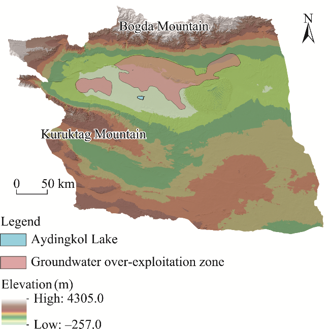
Fig. 1 Terrain and elevation of Turpan City

2.2 Data sources

The datasets and their sources used in this study are listed in Table 1, including land use, topographic, climatic, and socio-economic dimensions. We classified the land use types of the study area into six categories: cultivated land, forest land, grassland, water body, construction land, and unused land, according to the land use classification scheme of the Chinese Academy of Sciences (Chen et al., 2023). The topographic, climatic, and socio-economic data as well as the information on the locations of reservoirs and driven wells collected by the Third Scientific Expedition to Xinjiang were used to the driving factor analysis. All vector and raster data employed in this study adhered to the World Geodetic System 1984 geographic coordinate system, and the projection coordinate system was standardized to Krasovsky_1940_Albers.
Table 1 Indicators and their data sources
Data type Indicator Period Resolution (m) Data source
Land use Land use type 2000-2020 30 https://www.resdc.cn
Topographic factor Digital elevation model (DEM) 2000-2020 30 https://www.gscloud.cn
Slope 2000-2020 30 https://www.gscloud.cn
Soil type 2000-2020 30 https://www.resdc.cn
Climatic factor Temperature 2000-2020 30 https://www.resdc.cn
Precipitation 2000-2020 30 https://www.resdc.cn
Socio-economic factor Population 2000-2020 30 https://www.resdc.cn
Gross domestic product rating (GDPR) 2000-2020 30 https://www.resdc.cn
Distance from government (DFG) 2000-2020 30 https://www.openstreetmap.org
Distance from primary road (DFPR) 2000-2020 30 https://www.openstreetmap.org
Distance from secondary road (DFSR) 2000-2020 30 https://www.openstreetmap.org
Distance from tertiary road (DFTR) 2000-2020 30 https://www.openstreetmap.org
Distance from riverbed (DFRD) 2000-2020 30 https://www.openstreetmap.org
Distance from reservoir (DFR) 2000-2020 30 https://www.xjsedata.cn
Distance from driven well (DFDW) 2000-2020 30 https://www.xjsedata.cn

3 Methodology

To obtain accurate ecological risk predictions of Turpan City under the business as usual (BAU), rapid economic development (RED), ecological protection priority (EPP), and ecological-economic balance (EEB) scenarios in 2030, we undertaken the follow steps. Step 1: selecting the dataset with the highest correlation to the prediction year of 2030 as the foundational data for PLUS model prediction by grey relational analysis. Step 2: predicting land use under four scenarios in 2030 by MOP-PLUS model involving 14 driving factors (digital elevation model (DEM), slope, soil type, temperature, precipitation, population, gross domestic product rating (GDPR), distance from government (DFG), distance from primary road (DFPR), distance from secondary road (DFSR), distance from tertiary road (DFTR), distance from riverbed (DFRD), distance from reservoir (DFR), and distance from driven well (DFDW)). Step 3: constructing the ecological risk evaluation system that includes four dimensions of urban construction pressure, landscape ecological risk, production pressure, and ecological degradation pressure to calculate the ecological risk level (ERL) of each land use type and the ERI of optimal grid scale. Step 4: utilizing spatial autocorrelation to investigate the spatial distribution characteristics of ERI. And step 5: clarifying the explanatory power of the driving factors to ecological risk and the interaction between driving factors through Geodetector; the driving factors of ecological risk included slope, soil type, temperature, precipitation, population, GDPR, DFG, DFPR, DFSR, DFTR, DFRD, DFR, and DFDW.

3.1 Grey relation analysis

The land use raster data of 2000, 2010, and 2020 were used as the primary grid data, while the corresponding annual datasets comprising topographic, climatic, and socio-economic raster data were employed as the comparative grid data. The mean grey relational coefficient for each pixel value in the main grid and the final overall mean grey relational coefficient were calculated using Equations 1-3 (Deng, 2019). This process was implemented using Python v.3.12.
$ \operatorname{GRC}_{(x, y)}=\frac{\Delta_{\min }+0.5 \times \Delta_{\max }}{\Delta+0.5 \times \Delta_{\max }},$
where GRC(x,y) is the grey relational coefficient; x and y denote the pixel values in the standardized primary raster data and the comparative raster data, respectively; Δ is the absolute difference between x and y; and Δmax and Δmin are the maximum and minimum absolute values of pixel value differences across all pixel locations, respectively.
$ \text { Ave } \operatorname{GRC}_{(v)}=\frac{1}{N_{v}} \sum_{i=1}^{N_{v}} \mathrm{GRC}_{i},$
$ \text { Ave } \operatorname{GRC}=\frac{1}{6} \sum_{v=1}^{6} \text { Ave } \operatorname{GRC}_{(v)}$
where Ave GRC(v) is the mean grey relational coefficient of pixels with a value of v within the main grid; v denotes all possible pixel values within the primary raster data; Ave GRC is the arithmetic mean of the average GRC(v) values; Nv is the total number of pixels in the main grid data with a value of v; and GRCi is the grey relational coefficient of the ith pixel. The main grid data are land use data, with the following values: cultivated land=1, forest land=2, grassland=3, water body=4, construction land=5, and unused land=6.

3.2 Multi-scenario settings

Four scenarios (BAU, RED, EPP, and EEB) were used to simulate the land use pattern of Turpan City in 2030. The primary distinction among these scenarios lies in the severity of ecological requirements and the pace of urban development. The area of each land use type used in this study was determined by the urban development planning objectives. In addition, all four scenarios were imposed spatial limitations that the transformation of water bodies into other land types were prohibited, while permitting the conversion of the remaining five land use types into water bodies, because of the crucial ecological value of water bodies in Turpan City.

3.2.1 Objective functions

We chose two optimization objectives, ecological benefit and economic benefit, based on the features of the study area and the difficulties of data quantification. The economic benefit objective function F1(x) and ecological benefit objective function F2(x) are calculated as follows (Chen et al., 2020):
$ F_{1}(x)=531.93 x_{1}+129.85 x_{2}+8.90 x_{3}+16.62 x_{4}+7412.39 x_{5}+0.00 x_{6} \text {, }$
$ F_{2}(x)=130.03 x_{1}{ }^{\prime}+411.18 x_{2}{ }^{\prime}+136.24 x_{3}{ }^{\prime}+865.07 x_{4}{ }^{\prime}+0.83 x_{5}{ }^{\prime}+7.90 x_{6}{ }^{\prime} \text {, }$
where x1 is the economic value of cultivated land (104 CNY/km2); x2 is the economic value of forest land (104 CNY/km2); x3 is the economic value of grassland (104 CNY/km2); x4 is the economic value of water body (104 CNY/km2); x5 is the economic value of construction land (104 CNY/km2); x6 is the economic value of unused land (104 CNY/km2); x1' is the ecological value of cultivated land (104 CNY/km2); x2' is the ecological value of forest land (104 CNY/km2); x3' is the ecological value of grassland (104 CNY/km2); x4' is the ecological value of water body (104 CNY/km2); x5' is the ecological value of construction land (104 CNY/km2); and x6' is the ecological value of unused land (104 CNY/km2).
The average land economic value of each land use type in 2020 was determined by the statistical yearbook (TMLCCC, 2021). The economic benefit coefficient of unused land was set to zero because of its extremely low economic benefits. We adopted the equivalent factor method to determine the ecological benefit coefficient of each land use type based on the statistical yearbook ''Compilation of National Agricultural Product Cost and Benefits Data'' (NDRC, 2015-2020) and the equivalent table of ecosystem service value per unit area examined by Xie et al. (2017).

3.2.2 Scenario definition

BAU scenario: this scenario serves as the baseline in which no land planning policies or resource constraints are taken into account. We assumed that the socio-economic and land evolution trends remain unchanged from 2020 to 2030 under the BAU scenario. We used the Markov-PLUS model to calculate the area of each land use type under the BAU scenario in 2030 based on a probability matrix of land use from 2010 to 2020.
RED scenario: economic development is prioritized over ecological protection under the RED scenario, requiring the optimal allocation of land cover structure to maximize the F1(x) objective. To ensure that the future land use changes comply with the law of natural development, we established the area of each land use type by referring the previous land cover area levels (TMLCCC, 2021). Under the RED scenario, the area of cultivated land in Turpan City was set as more than 1303.75 km2, which is the area of cultivated land in 2020. The area of forest land was set as more than 76.42 km2, which is the area of forest land under the BAU scenario. The area of grassland was set as 10,553.03-10,599.55 km2, of which the lower limit is the area of grassland in 2020, while the upper limit is the area of grassland under the BAU scenario. The area of water body was set as more than 60.18 km2, which is the area of water body in 2020. The area of construction land was set as more than 405.81 km2, which is the area of construction land in 2020. The area of unused land was set as 56,793.95-56,564.37 km2, of which the upper limit is the area of unused land in 2020, while the lower limit is the area of unused land in 2000 (Yuan et al., 2024).
EPP scenario: ecological protection is prioritized over economic development under the EPP scenario, requiring the optimal allocation of land cover structure to maximize the F2(x) objective. According to the above-mentioned definition of EPP scenario, we set the range of the areas of cultivated land, water body, construction land, and unused land under the EPP scenario, the same as them under the RED scenario. At the same time, restrictions on the areas of forest land and grassland were relaxed to counterbalance the expansion of these four land use types. The area of forest land was set as more than 80.86 km2 under the EPP scenario, which is the area of forest land under the BAU scenario. The area of grassland was set as more than 10,553.03 km2, which is the area of grassland in 2020.
Considering the ecological need for windbreak and sand fixation, the ratio of the sum of the areas of forest land and grassland to the sum of the areas of construction land and unused land in 2020 was taken as the lower limit under the EPP scenario (Wang et al., 2023):
$ \frac{s_{2}+s_{3}}{s_{5}+s_{6}} \geq 0.19$,
where s2 is the area of forest land (km2); s3 is the area of grassland (km2); s5 is the area of construction land (km2); and s6 is the area of unused land (km2).
EEB scenario: to balance economic development with regional ecological benefits, the optimal distribution of land cover quantity structure requires the maximization of these two objectives at the same time. The formula is as follows:
$ \operatorname{Max}\left\{F_{1(x)}, F_{2(x)}\right\}=a F_{1(x)}+b F_{2(x)}$
where Max{F1(x), F2(x)} is the comprehensive maximum value of ecological benefits and economic benefits; a is the economic benefit weight value; and b is the ecological benefit weight value. According to the future development orientation of the study area and expert opinions, we set a=0.40 and b=0.60 in this study. We set the areas of all the six land use types under the EEB scenario, the same as them under the EPP scenario. Besides, according to the definition of EEB scenario, we set the other three constraints on the area of different land use types:
$ \frac{s_{5}}{s_{1}} \geq 0.31$
$ \frac{s_{4}}{s_{1}} \geq 0.05$
$ s_{2}+s_{3} \geq 10,636.01$
where s1 is the area of cultivated land (km2); and s4 is the area of water body (km2).
As required by the theoretical environmental criteria, the sum of the areas of forest land and grassland under the EEB scenario cannot be less than the sum of the areas of the two land use types under the BAU scenario. The LINGO v.18.0 software (Lindo System Inc., Chicago, Illinois, USA) was used to solve the above formulas combined with constraints.

3.3 Ecological risk assessment

By comparing the spatial distribution characteristics of ERL at different spatial scales of 3 km×3 km, 4 km×4 km, 5 km×5 km, 6 km×6 km, and 7 km×7 km, we found that the distribution of ERL at the grid size of 6 km×6 km had a strong correlation with land use data. Therefore, a 6 km×6 km grid was selected as the unit.
As shown in Table 2, the urban expansion intensity (UEI) and land-use composite index (LUCI) were selected to assess the urban expansion pressure (Guo et al., 2024). The proportion of cultivated land within productive and living land (PCL) and the proportion of economic land (PEL) across the whole land were employed to assess the production pressure associated with landscape ecological risk (Yu et al., 2023). The Shannon's diversity index (SHDI) and landscape disturbance index (LDI) were chosen as evaluation indicators for the landscape ecological risk (Hossen and Sultana, 2024). The ecological capability (EC), ecological service value (ESV), and the proportion of ecological land (PEC) across the whole land were chosen to assess ecological degradation pressure (Luo et al., 2018). The 9 indicators constructed a comprehensive ecological risk evaluation system. We used the analytic hierarchy process analytic hierarchy process (AHP) method to determine the hierarchical analysis weight and the technique for Order Preference by Similarity to an Ideal Solution (TOPSIS) method for determining the entropy method weight of each indicator, and then applied Equation 11 to calculate the combined weight of each indicator (Gao et al., 2022):
$ b_{j}=\frac{\mathrm{AP}_{j} \times \mathrm{TP}_{j}}{\sum_{j=1}^{m=9} \mathrm{AP}_{j} \times \mathrm{TP}_{j}},$
where bj is the combined weight of the jth ecological risk evaluation indicator; APj is the hierarchical analysis weight of the jth indicator; TPj is the entropy method weight of the jth indicator; and m is the number of indicators.
Table 2 Weight of each indicator used for ecological risk assessment
Evaluation category Indicator Hierarchical analysis weight Entropy method weight Combined weight
Urban expansion pressure UEI 0.3688 0.0939 0.2841
LUCI 0.1288 0.2048 0.2066
Production pressure PCL 0.0362 0.0759 0.0226
PEL 0.1085 0.1612 0.1437
Landscape ecological risk SHDI 0.0907 0.2170 0.1617
LDI 0.1814 0.0953 0.1421
Ecological degradation pressure EC 0.0543 0.0537 0.0240
ESV 0.0232 0.0503 0.0096
PEC 0.0147 0.0478 0.0058

Note: UEI, urban expansion intensity; LUCI, land use composite index; SHDI, Shannon's diversity index; LDI, landscape disturbance index; PCL, proportion of cultivated land within productive and living land; PEL, proportion of economic land across the whole land; EC, ecological capability; ESV, ecological service value; PEC, proportion of ecological land across the whole land.

We used Equations 12 and 13 to calculate the ERL of each land use type and ERI of each 6 km×6 km grid.
$ \mathrm{ERL}_{i}=\sum_{i=1}^{n=6} \sum_{j=1}^{m=9} a_{i j} b_{j},$
$ \mathrm{ERI}=\sum_{i=1}^{n=6} \mathrm{ERL}_{i} \frac{\mathrm{~s}_{i}}{M},$
where i (i=1, 2, 3, 4, 5, and 6) is the land use type, of which 1 represents cultivated land, 2 represents forest land, 3 represents grassland, 4 represents water body, 5 represents construction land, and 6 represents unused land; j (j=1, 2, 3, 4, 5, 6, 7, 8, and 9) is the indicators used for ecological risk assessment, of which 1 represents UEI, 2 represents LUCI, 3 represents SHDI, 4 represents LDI, 5 represents PCL, 6 represents PEL, 7 represents EC, 8 represents ESV, and 9 represents PEC; ERLi is the ecological risk level of the ith land use type; aij is the normalized weight of the jth ecological risk evaluation indicator in the ith land use type; n is the number of land use types; si is the area of the ith land use type in one grid (km2); and M is the area of grid (km2). In this study, M equals to 36.00 km2.
The calculations of the indicators of UEI, LUCI, LDI, PCL, PEL, EC, ESV, and PEC are shown in Equations 14-21:
$ \mathrm{UEI}=\frac{\Delta U}{I \times 10},$
where ΔU is the change in the area of construction land per decade (km2); and I is the area of construction land of the first year in every decade (i.e., 1990, 2000, 2010 in this study) (km2).
The LUCI reflects the extent of human exploitation of land, serving as a crucial indicator for measuring both the depth and breadth of regional land use (Montejano Escamilla et al., 2016):
$ \mathrm{LUCI}=100 \times \sum_{i=1}^{n=6}\left(V \times C_{i}\right),$
where V is the value of land use type, where unused land equals to 1, forest land, grassland, and water body equal to 2, cultivated land equals to 3, and construction land equals to 4; and Ci is the ratio of the area of the ith land use type to the total area across all land use types.
$ \mathrm{LDI}=0.5 \mathrm{PD}+0.3 \mathrm{DI}+0.2 \mathrm{SI},$
where PD is the patch density (patch number/100 hm2); DI is the landscape division and is used to describe the degree of landscape fragmentation; and SI is the splitting index, used to assess landscape connectivity. The proportions of the three indices in the LDI were determined by referring to Cheng et al. (2023). Fragstats v.4.2 (University of Massachusetts Amherst, Amherst, Massachusetts, USA) was used to calculate the PD, DI, SI, and SHDI.
$ \mathrm{PCL}=\frac{s_{1}}{\sum_{i=1}^{n=5} s_{i}},$
$ \text { PEL }=\frac{S_{1}+s_{5}}{\sum_{i=1}^{n=6} s_{i}},$
$ \mathrm{EC}=\sum_{1}^{6} s_{i} \times r_{i} \times y_{i},$
$ \mathrm{ESV}=\sum_{1}^{6} s_{i} \times A C_{i},$
$ \mathrm{PEC}=\frac{s_{2}+s_{3}+s_{4}}{\sum_{i=1}^{i=6} s_{i}},$
where si is the area of each land use type (km2); ri is the equilibrium factor; yi is the production factor; and ACi is the ecological service value per pixel of the ith land use type (CNY/km2) (Tong et al., 2023).

3.4 Spatial autocorrelation analysis

Global spatial autocorrelation analysis (global Moran's I index) was initially employed to validate the spatial correlation of ERI (Li et al., 2022a). The formula for calculating the global Moran's I index is given in Equation 22.
$ \text { Moran's } I=\frac{l \sum_{i=1}^{l} \sum_{j=1}^{l} W_{i j}\left(x_{i}-\bar{x}\right)\left(x_{j}-\bar{x}\right)}{\sum_{i=1}^{l} \sum_{j=1}^{l} W_{i j} \sum_{i=1}^{n}\left(x_{i}-\bar{x}\right)^{2}},$
where l is the total number of observations; xi and xj are the observed values at locations i and j, respectively; $ \bar{x}$ is the mean observed value of all locations, providing a reference point for measuring deviations in individual observations; and Wij is the spatial weight between locations i and j, typically derived from an adjacency matrix that defines the spatial relationships between pairs of locations. The $ \sum_{i=1}^{l} \sum_{j=1}^{l} W_{i j}$ is the sum of all spatial weights, standardizing the overall spatial interaction in the dataset to account for varying numbers of neighbors or differing proximity between locations.
The global Moran's I index ranges from -1 to 1. The Moran's I>0 indicates a spatially positive correlation in ERI, with higher values indicating stronger agglomeration. Conversely, the Moran's I<0 indicates a negative spatial correlation, and closer to -1 signifies stronger dispersion. Finally, the Moran's I=0 denotes no spatial correlation. In this study, according to the spatial correlation of ERI, we obtained high-high, low-low, low-high, high-low, and non-significant five ecological risk clusters. The high-high clusters denote areas of high-value concentration, where both the ecological risk and the risk levels of adjacent regions are elevated. This pattern often reflects similar environmental pressures across these areas, making them a priority for ecological management (Li et al., 2020). Enhanced governance measures should be considered for these areas. The low-low clusters denote areas with concentrated low values, encircled by other low-risk areas. These areas typically reflect stable ecosystems, and it is advisable to retain current management practices to prevent any increase in risk (Folke et al., 2010). The low-high clusters denote areas with relatively low risk, adjacent to areas with higher risk levels. These areas could become potential areas for the transfer of environmental pressures in the future, requiring close attention to prevent ecological deterioration driven by external pressures (Seitzinger et al., 2005). The high-low clusters indicate areas with high internal risk, surrounded by areas with lower risk levels. This pattern suggests the presence of isolated environmental challenges or localized ecological pressures (Li et al., 2023). Strategies for these areas should prioritize targeted restoration efforts and mitigation of potential spillover effects on adjacent areas. The non-significant clusters indicate that the spatial clustering in these areas is not significant, suggesting that the ecological risk levels do not exhibit a clear spatial pattern.
We employed the Getis-Ord Gi* index to unveil the spatial distribution patterns of areas exhibiting high and low values of ERI:
$ G_{i}^{*}=\frac{\sum_{j=1}^{l} W_{i j} x_{j}-\bar{x} \sum_{j=1}^{l} W_{i j}}{\sqrt{\frac{\sum_{j=1}^{l} x_{j}^{2}}{l}-(\bar{x})^{2} \sqrt{\frac{\left[\sum_{j=1}^{l} W_{i j}^{2}-\left(\sum_{j=1}^{l} W_{i j}\right)^{2}\right]}{l-1}}},}$
where Gi* is the Getis-Ord Gi* index. Getis-Ord Gi* analysis measures the concentration ratio based on Z-score identified as high (positive Z-values) and low values (negative Z-values). Z-score>2.58 indicates an extremely hot area at 99% confidence level, while 1.96<Z-score<2.58 signifies a hot area at 95% confidence level (Getis and Ord, 1992).

3.5 Geographical detector method

Geodetector is a statistical tool that facilitates the detection of spatial differentiation and identification of underlying driving forces, with the ability to analyze both quantitative and qualitative data and investigate the impact of individual factors or their interactions on dependent variables (Liu et al., 2022). The magnitude of the influence of each driving factor on the dependent variable ERI change was measured by q-value, and the formula is as follows:
$ q=1-\frac{\sum_{h=1}^{L} N_{h} \sigma_{h}^{2}}{N \sigma_{h}^{2}},$
where q is the influence of a single driving factor on ERI change q $ \in$ [0,1]; h is the number of layers; L is the stratification of driving factor; Nh and N are the sample size of a stratum and the whole region, respectively; and σ2 hand σ2 are the sum of variance of a stratum and the whole region, respectively. The larger the value of q, the greater the influence of driving factor on ERI change.

4 Results

4.1 Dynamic evolution of land use

4.1.1 Dynamic evolution of land use from 2000 to 2020

With the implementation of the Western Development Strategy and the promotion of water-saving irrigation technology, land use from 2000 to 2020 has undergone significant changes. The areas of cultivated land and construction land increased by 52.30% and 75.02% from 2000 to 2010, respectively, which was the most obvious change, followed by an increase in the areas of grassland and water body by 21.31% and 37.23%, respectively. The areas of forest land and unused land decreased by 53.95% and 3.92%, respectively. In terms of spatial distribution, in the central basin, there was a significant increase in cultivated land and construction land from 2000 to 2010 (Fig. 2). It is worth noting that the central basin is dotted with newly driven wells. Interconversion of intermountain grassland and unused land was evident in the northern and southwestern parts of Turpan City. The area of land use type change from 2010 to 2020 was significantly less than that in the last decade. The area of construction land increased by 62.54% from 2010 to 2020, the areas of grassland and water body increased by 0.08% and 17.01%, respectively, whereas the areas of cultivated land, forest land, and unused land decreased by 3.30%, 18.51%, and 0.19%, respectively. In terms of spatial distribution, land use changes from 2010 to 2020 were mainly concentrated in the central basin, and the number of new driven wells built in this region was much higher than the total number of driven wells during 2000-2010, as well as new reservoirs to the west and north within the perimeter. In addition, water bodies have been added to the unused land in the southeast part of the basin.
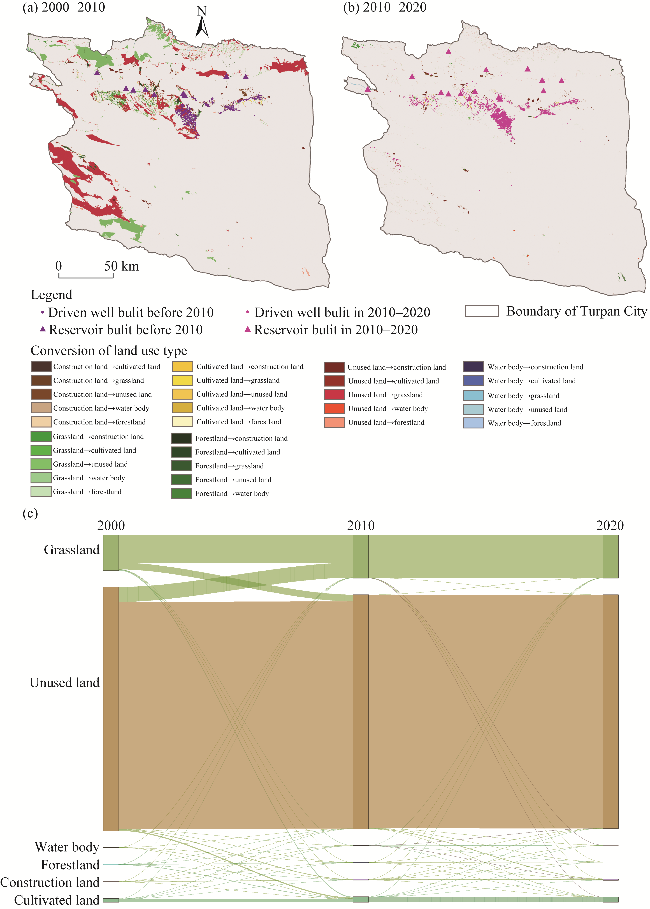
Fig. 2 Land use transition in Turpan City from 2000 to 2020. (a), spatial distribution of land use transition from 2000 to 2010; (b), spatial distribution of land use transition from 2010 to 2020; (c), diagram of land use transition from 2000 to 2020. In Figure 2c, the width of colored block represents the area of the corresponding land use type; the curve represents the transition between two land use types; the width of curve represents the transition area between two land use types, and the wider the curve, the larger the transition area.

4.1.2 Driving factor of land use change

The contribution of each driving factor to land use change was similar for cultivated land, construction land, and unused land during 2000-2010 (Fig. 3). For all the six land use types, the driving factor of DEM has the highest contribution rate to land use change from 2000 to 2020. For cultivated land, the driving factors of DEM (19.98%), DFDW (17.90%), and GDPR (10.34%) contributed the most to its conservation from 2000 to 2020. For forest land, from 2000 to 2010, the driving factor of DFPR had a high contribution rate (14.17%), while from 2010 to 2020, the driving factor of DFTR had a high contribution rate (14.26%); both DFPR and DRTR were socio-economic factors. For grassland, the temperature contributed more to its conversion from 2010 to 2020 (16.88%). For water body, the driving factors of DFR and DFRD had a great contribution to its conservation from 2000 to 2020, except for DEM. For construction land, the driving factors of temperature, DFPR, and DFDW had higher contribution rates than others. For unused land, which had the largest area in Turpan City, the driving factors of GDPR and DFDW contributed more to its conversion than others from 2000 to 2020. The driving factor of DFSR experienced significant increase on the conversion of unused land from 2010 to 2020. From Figure 4 we can see that the primary driving factors of land use change in Turpan City from 2000 to 2020 were socio-economic factors, except for DEM and temperature.
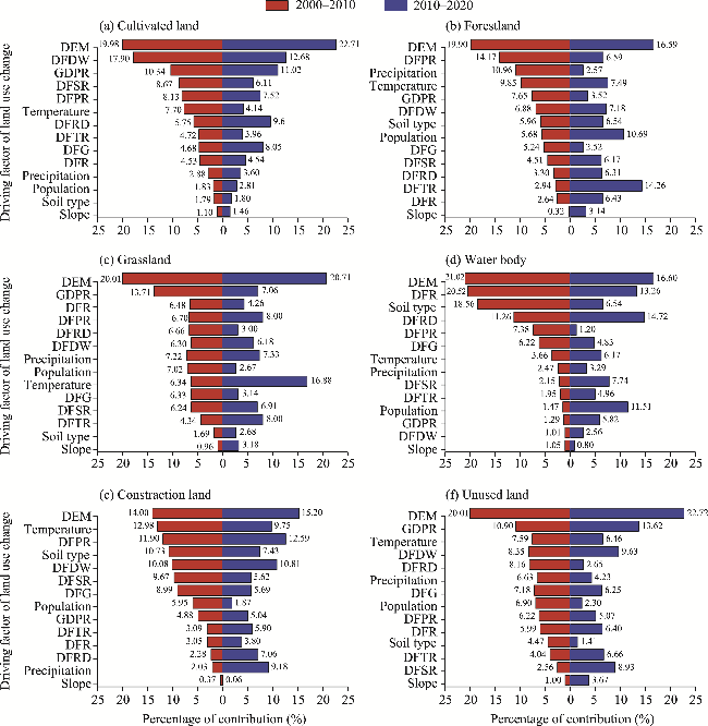
Fig. 3 Proportion of the contribution of each driving factor to land use transition from 2000 to 2020. (a), cultivated land; (b), forest land; (c), grassland; (d), water body; (e), construction land; (f), unused land. DEM, digital elevation model; GDPR, gross domestic product rating; DFG, distance from government; DFRD, distance from riverbed; DFR, distance from reservoir; DFDW, distance from driven well; DFPR, distance from primary road; DFSR, distance from secondary road; DFTR, distance from tertiary road.

4.1.3 Spatial distribution of land use in 2030

We validated the land use of Turpan City in 2020, which was simulated by PLUS model based on land use data of 2000 and 2010 against actual data. The Kappa coefficient was 0.895 and the overall accuracy was 0.971, indicating high accuracy. The simulation results confirmed the reliability of PLUS model. Combining the 2020 land use data with the MOP model parameters, land use in 2030 was modeled under different scenarios (Fig. 4).
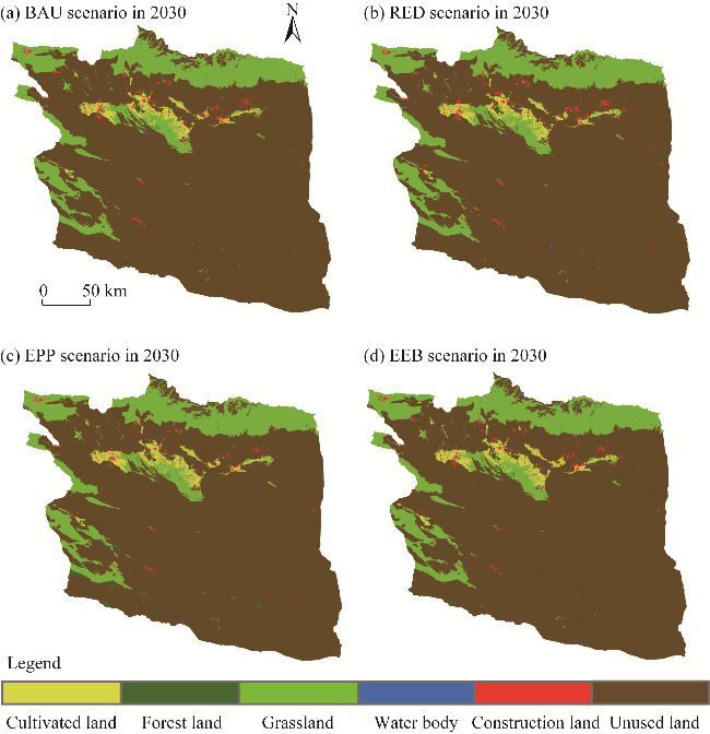
Fig. 4 Spatial distribution of land use types under different scenarios in 2030. (a), business as usual (BAU) scenario; (b), rapid economic development (RED) scenario; (c), ecological protection priority (EPP) scenario; (d), eco-economic equilibrium (EEB) scenario.
The area of different land use types in 2030 under different scenarios is shown in Table 3. The area of grassland did not change in the RED, EEB, and EPP scenarios, except for the BAU scenario. The BAU and RED scenarios showed a significant increase in the area of construction land by 30.79% and 57.67%, respectively. The areas of cultivated land, forest land, and unused land under the BAU scenario decreased by 2.89%, 5.49%, and 0.17%, respectively, while the areas of water body and grassland increased by 10.39% and 0.06%, respectively. There was no change in the cultivated land, grassland, and water body under the RED scenario, and the area of forest land decreased by 5.49%. The area of construction land under the EPP scenario did not increase, but the areas of cultivated land, forest land, and water body increased by 0.41%, 235.54%, and 56.18%, respectively. Under the EEB scenario, the areas of cultivated land, forest land, water body, and construction land increased by 12.64%, 2.62%, 22.02%, and 12.18%, respectively.
Table 3 Area and change percentage of each land use type under different scenarios in 2030
Land use type BAU scenario RED scenario EPP scenario EEB scenario
Area
(km2)
Percentage (%) Area
(km2)
Percentage (%) Area (km2) Percentage (%) Area (km2) Percentage (%)
Cultivated land 1266.12 -2.89 1303.75 0.00 1309.07 0.41 1468.54 12.64
Forest land 76.42 -5.49 76.42 -5.49 271.32 235.54 82.98 2.62
Grassland 10,559.59 0.06 10,553.03 0.00 10,553.03 0.00 10,553.03 0.00
Water body 66.43 10.39 60.18 0.00 93.99 56.18 73.43 22.02
Construction land 530.74 30.79 639.84 57.67 405.81 0.00 455.25 12.18
Unused land 56,698.28 -0.17 56,564.37 -0.40 56,564.37 -0.40 56,564.37 -0.40

Note: BAU, business as usual; RED, rapid economic development; EEP, ecological protection priority; EEB, eco-economic equilibrium. The percentage represents the change rate of the area of each land use type in 2030 compared with that in 2020, of which positive percentage means increase, while negative percentage means decrease.

Influenced by the LEAS-generated growth probability for each land use type in each grid, the distribution of land use type in Turpan City under the four scenarios in 2030 was similar to that in 2020 (Fig. 4). The change of forest land mainly occurred in the southwestern part of Turpan City, the change of water body mainly occurred in the southeastern part, and the changes of cultivated land and construction land were concentrated in the central basin.

4.2 Ecological risk

4.2.1 Ecological risk in the whole region

The ERL of different land use types for all scenarios in this study are listed in Table 4. The value of ERL for each land use type was unused land>grassland>cultivated land>construction land>forest land>water body. The value of ERL of unused land was significantly higher than that of other land types, mainly because the area of unused land was high, resulting in a significantly higher value of LUCI than those of other land use types. The overall ecological environment did not improve significantly from 2010 to 2020 (Table 4). In 2030, the order of ecological risk from the highest to lowest was RED>BAU>EEB>EPP (Table 4).
Table 4 Value of ecological risk level (ERL) of each land use type in Turpan City in 2000, 2010, 2020, and 2030 under four scenarios
Land use type ERL
2000 2010 2020 2030
BAU scenario RED scenario EPP scenario EEB scenario
Cultivated land 0.1443 0.1822 0.1802 0.1749 0.1852 0.1704 0.1779
Forest land 0.1147 0.1441 0.1423 0.1373 0.1471 0.1356 0.1380
Grassland 0.1982 0.2428 0.2421 0.2378 0.2472 0.2324 0.2364
Water body 0.1107 0.1432 0.1418 0.1369 0.1466 0.1323 0.1376
Construction land 0.1160 0.1505 0.1543 0.1538 0.1669 0.1443 0.1507
Unused land 0.3208 0.3524 0.3509 0.3461 0.3558 0.3412 0.3467
To visually analyze the spatial distribution characteristics of ecological risk, we used the natural breakpoint method to classify the ERI into seven levels: I (ERI≤0.2191), II (0.2191<ERI≤0.2548), III (0.2548<ERI≤0.2831), IV (0.2831<ERI≤0.3086), V (0.3086<ERI≤0.3301), VI (0.3301<ERI≤0.3453), and VII (ERI>0.3453) (Table 5; Fig. 5).
Table 5 Proportion of area at each level of ecological risk index (ERI) in Turpan City in 2000, 2010, 2020, and 2030 under four scenarios
Level of ERI Proportion of area (%)
2000 2010 2020 2030
BAU scenario RED scenario EPP scenario EEB scenario
I 8.46 1.28 1.50 1.73 1.39 1.95 1.78
II 4.62 8.85 8.75 9.14 8.13 9.69 9.47
III 3.56 4.62 4.79 5.02 4.62 4.96 4.73
IV 4.68 3.79 4.12 4.63 4.29 5.29 4.73
V 78.67 5.01 5.01 5.18 5.52 6.02 5.07
VI 0.00 5.01 5.52 10.14 4.46 72.09 8.74
VII 0.00 71.44 70.31 64.16 71.59 0.00 65.48
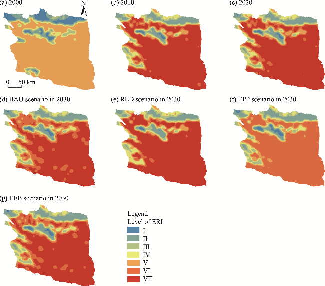
Fig. 5 Spatial distribution of ecological risk in Turpan City. (a), 2000; (b), 2010; (c), 2020; (d), BAU scenario in 2030; (e), RED scenario in 2030; (f), EPP scenario in 2030; (g), EEB scenario in 2030. ERI, ecological risk index.
Overall, the ERI increased rapidly from 2000 to 2010, accompanied by large area conversion from unused land to water body in the southeastern part of Turpan City and the development of construction land in the southwestern part. Under the BAU, RED, EPP, and EEB scenarios, the proportions of the area at VI and VII levels were 74.30%, 76.05%, 72.09%, and 74.22%, respectively, which decreased by 1.53%, increased by 1.75%, decreased by 3.96%, and increased by 2.13%, respectively compared with 2020. Under the EPP scenario, the proportion of the area at VII level was zero, mainly due to the decrease in intensity of urban expansion and the increase of ecological land coverage. Notably, ecological evaluation units with a large proportion of unused land had higher ecological risk under the four scenarios. Therefore, when unused land in an ecological unit was converted into water body or construction land, the ecological risk to the ecological unit decreased rapidly. Under the BAU, RED, and EEB scenarios, the ERL decreased rapidly in new water bodies in the southeastern part of Turpan City and new construction land in the southwestern part.

4.2.2 Ecological risk in the goal region

The spatial distribution of ERI highlighted significant ecological changes, particularly in areas surrounding the Aydingkol Lake and areas experiencing groundwater over-exploitation (i.e., goal region of Turpan City). The ERI of the goal region was ranked in descending order as follows: RED in 2030>2010>2020>BAU in 2030>EEB in 2030>EPP in 2030>2000 (Table 6; Fig. 6).
Table 6 Proportion of area at each level of ERI in the goal region of Turpan City in 2000, 2010, 2020, and 2030 under four scenarios
Level of ERI Proportion of area (%)
2000 2010 2020 2030
BAU scenario RED scenario EPP scenario EEB scenario
I 15.14 12.43 13.51 15.76 13.04 17.93 16.22
II 15.68 15.14 14.59 15.22 13.59 14.67 16.22
III 14.05 11.35 12.43 11.96 13.04 13.04 11.35
IV 12.43 6.49 7.57 8.15 8.70 10.87 9.73
V 42.70 13.51 12.43 14.13 14.67 11.96 11.89
VI 0.00 11.35 13.51 18.48 5.98 31.52 17.84
VII 0.00 29.73 25.95 16.30 30.98 0.00 16.76
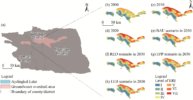
Fig. 6 Spatial distribution of ecological risk in the goal region of Turpan City. (a), the location of the goal region of Turpan City; (b), 2000; (b), 2010; (c), 2020; (d), BAU scenario in 2030; (e), RED scenario in 2030; (f), EPP scenario in 2030; (g), EEB scenario in 2030.
The proportion of area at I level, which represents the lowest ecological risk, decreased from 15.14% in 2000 to 12.43% in 2010, and recovered slightly to 13.51% in 2020. Similarly, the proportion of area at II level showed a decline from 15.68% in 2000 to 14.59% in 2020. Similarly, the proportion of area at IV level dropped significantly from 12.43% in 2000 to 7.57% in 2020. Notably, the proportion of area at V level, which reflects high ecological risk, began at 42.70% in 2000 and fell sharply to 12.43% in 2020.
The four scenarios in 2030 revealed different ecological risk in the goal region of Turpan City. Under the BAU scenario, the proportions of area at I, II, and III levels were expected to rise slightly, indicating a potential for recovery. However, the proportions of area at IV, V, and VI levels were projected to see marginal improvements, reflecting ongoing ecological stress; while the proportion of area at VII level declined sharply, indicating the recovery of environment in the goal region. Under the RED scenario in 2030, comparing with 2020 and the BAU scenario in 2030, the proportion of area at VI level decreased while the proportion of area at VII level increased, and the areas at other levels had slightly variation. Conversely, the proportion of area at VI level increased acutely while the proportion of area at VII level decreased to zero, indicating some success in conservation efforts. Ecological risk under the EEB scenario in 2030 showed almost same distribution with that in 2020.

4.3 Spatial-temporal characteristics of ecological risk cluster

The test of significance and calculation yielded a P-value<0.01 and a Z-score>2.58. Therefore, the spatial distribution pattern of ERI under all the four scenarios cannot be considered as the result of random processes. As shown in Figure 7, the global Moran's I value (>0.750) was positive for different time periods and scenarios in Turpan City, indicating a significant positive correlation of ERI in different time periods and under different scenarios. In addition, the scatter points were all close to the regression line and concentrated in the first and third quadrants, indicating that the ERI exhibited a clustered spatial distribution pattern.
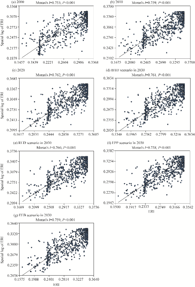
Fig. 7 Moran's I index scatterplot of ERI in Turpan City. (a), 2000; (b), 2010; (c), 2020; (d), BAU scenario in 2030; (e), RED scenario in 2030; (f), EPP scenario in 2030; (g), EEB scenario in 2030.
As shown in Figure 8, the ERI clusters in 2000, 2010, 2020, and 2030 (with four scenarios) were dominated by high-high and low-low clusters. It is worth noting that the spatial distribution of ecological risk was very similar, except in 2000. The similar spatial distribution was shown as follows: (1) the high-high aggregation areas were mainly distributed in the southwestern ecologically fragile areas, where unused land was the main land use type; (2) the low-low aggregation areas were mainly distributed in the central oasis basin and the mountainous areas in the northern part, where grassland was the main land use type; (3) the non-significant aggregation areas and high-low aggregation areas were regularly distributed near the boundary of the groundwater over-exploitation zone; and (4) the Aydingkol Lake was located in the non-significant area. These characteristics indicated a complex and unstable environment surrounding the over-exploitation areas. The ecological zone around the Aydingkol Lake was likely to remain in a prolonged state of instability, underscoring the need for immediate establishment of ecological buffer zones in these areas to ensure long term stability.
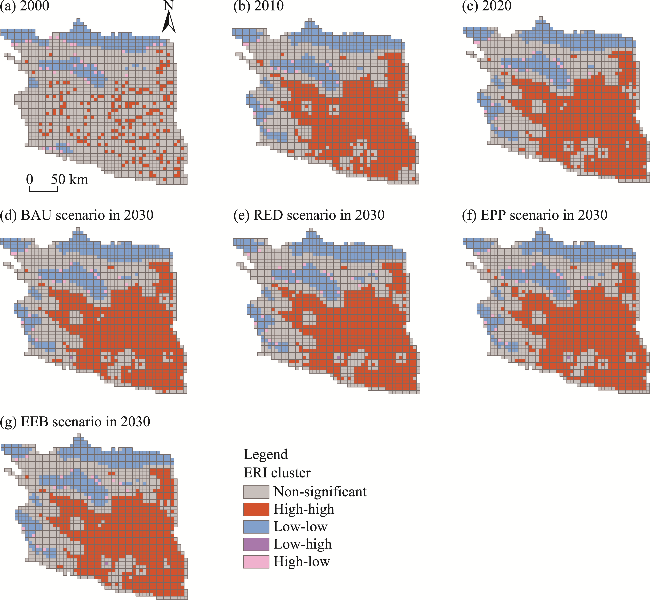
Fig. 8 Spatial distribution of ecological risk cluster in Turpan City. (a), 2000; (b), 2010; (c), 2020; (d), BAU scenario in 2030; (e), RED scenario in 2030; (f), EPP scenario in 2030; (g), EEB scenario in 2030.

4.4 Driving factors for ecological risk

4.4.1 Factor detector analysis

As shown in Table 7, the explanatory power and significance of the driving factors of ecological risk are provided. As shown in Figure 9, both in 2010 and 2020, the driving factors of GDPR, population, temperature, soil type, and precipitation had higher explanatory power to ecological risk. The GDPR consistently remained as the primary driving factor, while the slope had the lowest explanatory power. For the whole region of Turpan City, there were differences between 2010 and 2020 in the rankings of significant explanatory factors. The rank in 2010 was soil type>temperature>population>GDPR>precipitation>DFR>DFRD>DFSR>DFPR= DFG>DFDW>DFTR; while the rank in 2020 was GDPR>population>soil type>temperature> precipitation>DFR>DFRD>DFSR>DFG>DFPR>DFDW>DFTR. For the goal region, the rank in 2010 was GDPR>DFTR>soil type>precipitation>temperature>population>DFDW; while the rank in 2020 was GDPR>population>DFTR>soil type>precipitation>temperature>DFDW. The driving factors demonstrated stronger explanatory power for the whole region than for the goal region, and both GDPR and population showed rapid increase in their explanatory powers from 2010 to 2020.
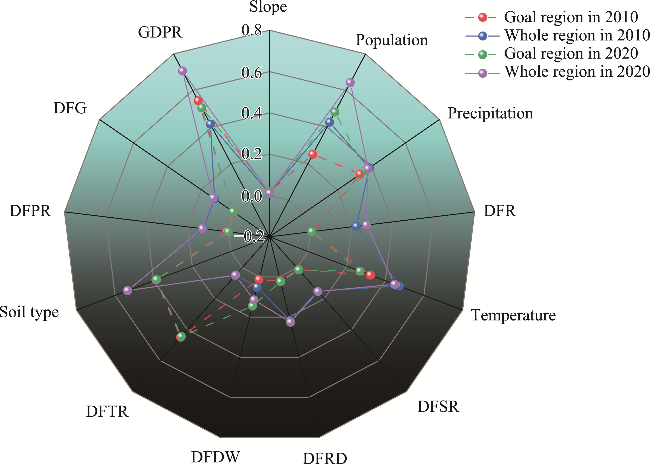
Table 7 Explanatory power (q) and significance (P) of each driving factor of ecological risk for the goal region and the whole region of Turpan City in 2010 and 2020
Driving factor 2010 2020
Goal region Whole region Goal region Whole region
q P q P q P q P
GDPR 0.543* 0.000 0.416* 0.000 0.505* 0.000 0.706* 0.000
Population 0.251* 0.000 0.426* 0.000 0.482* 0.000 0.643* 0.000
Precipitation 0.334* 0.000 0.388* 0.000 0.366* 0.000 0.380* 0.000
DFR 0.007 0.956 0.224* 0.000 0.006 0.964 0.273* 0.000
Temperature 0.322* 0.000 0.472* 0.000 0.269* 0.000 0.448* 0.000
DFSR 0.012 0.701 0.151* 0.000 0.014 0.652 0.154* 0.000
DFRD 0.020 0.324 0.218* 0.000 0.024 0.264 0.226* 0.000
Slope 0.018 0.924 0.010 0.024 0.017 0.941 0.011 0.011
DFTR 0.449* 0.000 0.047* 0.000 0.444* 0.000 0.049* 0.000
Soil type 0.388* 0.000 0.536* 0.000 0.385* 0.000 0.535* 0.000
DFPR 0.011 0.620 0.124* 0.000 0.001 0.740 0.128* 0.000
DFG 0.011 0.620 0.124* 0.000 0.014 0.548 0.131* 0.000
DFDW 0.133* 0.000 0.051* 0.000 0.145* 0.000 0.114* 0.000

Note: *, P<0.001 level.

Fig. 9 Explanatory power of each driving factor of ecological risk for the goal region and the whole region of Turpan City in 2010 and 2020

4.4.2 Factor interaction detection

As shown in Figure 10, in the goal region of Turpan City in 2010, the interactions between soil type and temperature, slope and precipitation, as well as population and GDPR were weak. In 2020, however, the interactions between those pairs were strong. In 2010, across the whole region, the interaction between population and DFTR was strong (0.661). In 2020, this interaction had further increased (0.673), and the interactions between GDPR and other driving factors were all over 0.700. The interactions between temperature and precipitation and between soil type and slope were weak. As shown in Figure 11, all the driving factors reinforced each other's explanatory power to ecological risk. In 2010, nonlinear interactions between factors were noticeably stronger than those in 2020. Specifically, in 2010, DFDW, DFG, DFPR, and slope displayed the most pronounced nonlinear enhancement with other factors. In contrast, slope and DFTR exhibited the most notable nonlinear interactions with other factors in 2020.
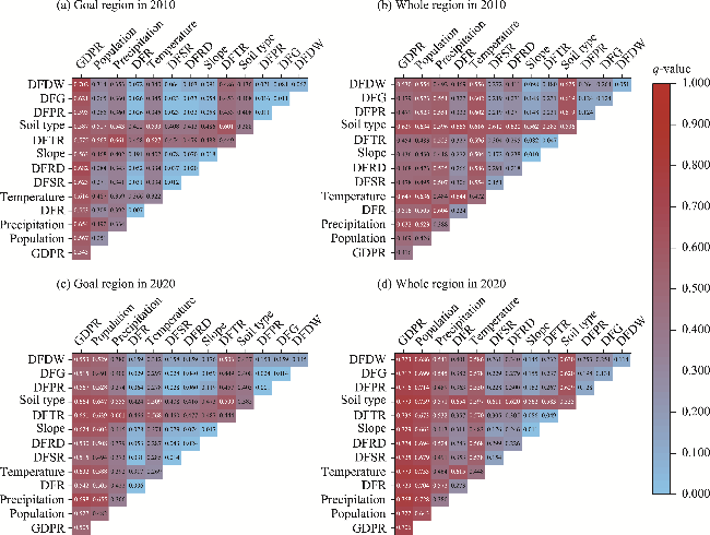
Fig. 10 Interactions between driving factor pairs of ecological risk in Turpan City in 2010 and 2020. (a), goal region in 2010; (b), whole region in 2010; (c), goal region in 2020; (d), whole region in 2020.
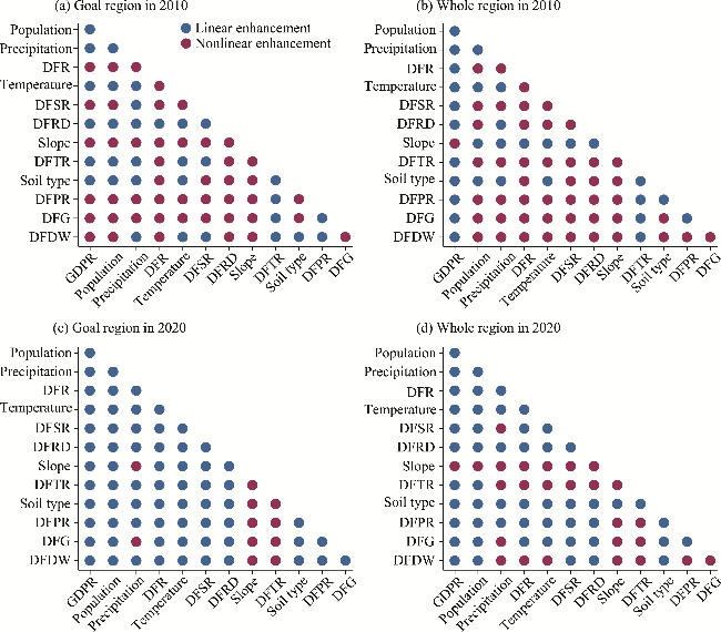
Fig. 11 Interaction patterns between driving factor pairs of ecological risk in Turpan City in 2010 and 2020. (a), goal region in 2010; (b), whole region in 2010; (c), goal region in 2020; (d), whole region in 2020.

5 Discussion

From 2000 to 2020, Turpan City experienced significant land use changes, mainly reflected in the expansion of cultivated land and construction land, as well as a decrease in unused land and forest land, which contributed to a substantial increase in ecological risk (Li et al., 2022b). Between 2000 and 2010, the expansion of cultivated land and construction land was primarily concentrated around newly established driven wells and reservoirs, which undeniably supported agricultural and urban development (Lee et al., 2022). However, the conversion of unused land into construction land and cultivated land, coupled with the reduction in forest land, has weakened the region's ecological buffering capacity (Zhou et al., 2023). According to the results of land driving contributions, excessive groundwater extraction has led to water resource shortages, which has significantly increased the environmental pressure from unused land development (Orme et al., 2015). Between 2010 and 2020, although the intensity of land use changes decreased, construction land continued to expand rapidly. Despite increases in grassland, water body, and cultivated land, forest land significantly diminished, along with a slowdown in the development of unused land (Cheng et al., 2023; Lin and Wang, 2023).
As unused land development slowed and new driven wells and reservoirs were introduced, the ERL of unused land decreased, resulting in an overall decline in ERL. The driving factor analysis of ecological risk showed that between 2000 and 2010, the rise in GDPR and population not only facilitated the expansion of construction land but also heightened ecological risks due to intensified human activities (Gan et al., 2023; Zhu and Cai, 2023). From 2010 to 2020, the natural terrain factors (slope and soil type) became more influential on ecological risk. However, the slightly reduction in the ERL of unused land from 2010 to 2020 driven by DFDW and DFR suggested that identifying alternative water sources is a beneficial human intervention that can mitigate adverse effects of land use changes (Corwin et al., 2022). For sustainable development, the exploration of new water resources is recommended to support regional development and construction efforts (Choudhary et al., 2021).
Within this study's framework, the contributions of various driving factors to land use transitions in future scenarios aligned with the pattern from 2010 to 2020. This means that the positive effects of DFDW and DFR on land conversion from 2010 to 2020 will persist under future scenarios (Liu et al., 2024). However, under the RED scenario, extensive conversion of construction land led to a significant increase in ERL, indicating that the current strategy of adding new driven wells and reservoirs to find alternative water sources is insufficient to meet the sustainability demands of the RED scenario (Dhakal et al., 2021). In contrast, under the other three future scenarios in 2030, the ERL of each land use type declined compared with 2020, suggesting that current water resource planning can support sustainable development under the BAU, EEB, and EPP scenarios (Xie et al., 2021).
The ecological risk in Turpan City was closely linked to the conversion of unused land into construction land and cultivated land. A significant increase in cultivated land (52.30%) and construction land (75.02%) was observed between 2000 and 2010, and a notable increase in construction land (62.54%) was observed from 2010 to 2020. Observing the environmental changes from 2000 to 2020 in Turpan City, the ecological risk increased sharply from 2000 to 2010 due to the rapid rise in urban sprawl pressure (Ye et al., 2024). The main driving factors of ecological risk were GDPR, population, soil type, and precipitation. Under the RED scenario in 2030, the area at high ecological risk was larger than the other scenarios. In future ecological management of Turpan City, emphasis should be placed on the rational allocation of water resources and sustainable land use, particularly for groundwater over-exploitation zones and the Aydingkol Lake (Inostroza et al., 2013). Therefore, managing groundwater over-exploitation zone should focus on controlling the unregulated expansion of construction land, especially by optimizing spatial layouts to reduce the dependence of construction land on groundwater (Tao et al., 2016). Restricting development permits for new construction land and encouraging land use shifts towards low-water ecological restoration are recommended. In terms of water resource management, advanced water-saving irrigation techniques such as drip and micro-irrigation should be incorporated to decrease groundwater consumption in agriculture. Additionally, the exploration of alternative water sources, including rainwater harvesting and recycled water, should be encouraged to reduce groundwater dependency (John et al., 2019).
Under the EPP scenario, increased forest land and water bodies have markedly improved the overall ecological environment, offering valuable insights for managing the Aydingkol Lake. The presence of low-low ecological risk clusters around the Aydingkol Lake suggested a certain recovery capacity in its natural ecosystem (Yang et al., 2024). Therefore, vegetation restoration projects around the Aydingkol Lake, such as planting drought-tolerant species suited to arid climates, are recommended to improve the local microclimate through increased vegetation cover, while mitigating soil erosion and desertification (Gao et al., 2024). Gradual restoration of natural ecological functions in the Aydingkol Lake can potentially reduce ecological risk in surrounding areas without intensifying water resource demands. For areas adapting to the BAU, EEB, and EPP scenarios, guiding land use toward ecological protection and restoration based on current water resource planning can help continually lower the ecological risk (Liu et al., 2015). Furthermore, given the positive impact of DFDW and DFR on land transformation, establishing a long-term monitoring system based on these driving factors in the goal region of Turpan City is advisable (Guo et al., 2022). Regularly monitoring the changes of ecological risk index in areas near driven wells and reservoirs will enable the assessment of environmental impact of water resource facilities, allow for timely adjustments to water resource development plans to ensure alignment with sustainable development goals in construction and development.

6 Conclusions

Based on the MOP-PLUS model, this study presented a novel ecological risk management framework, which closely related ecological risks and land use changes, for urban development in ecologically fragile regions. As the case study, this paper analyzed the changes in land use and ecological risk in Turpan City from 2000 to 2020, and set up four scenarios (BAU, RED, EPP, and EEB) to simulate the relevant data in 2030. The results showed that from 2000 to 2020, the area of unused land dramatically decreased, while the areas of grassland, construction land, and cultivated land increased. Under the four predicted scenarios in 2030, the area of unused land, which is the largest land use type located mainly in the southeastern part of the city, was decreased under all four scenarios, and the area of construction land increased due to urban expansion. The main factors influencing the land use change in Turpan City were DEM and socio-economic factors such as GDPR and DFDW, and the environment deteriorated. Comparing to 2020, the ERL of all six land use types decreased under the BAU, EPP, and EEB scenarios in 2030, except for the RED scenario. The reason for the difference is that the RED scenario emphasizes economic benefit more than environment benefit. The goal region of Turpan City, where lots of residents live, was mainly at I-V levels of ecological risk. The dominant driving factors of ecological risk were GDPR, soil type, population, temperature, and DFRD. The interactions between these driving factor pairs amplified their influence on ecological risk. Under the present planning and management of water resources, it was not sufficient to support the sustainable development under the RED scenario. Although there was some improvement in the ecological environment under the BAU and EPP scenarios, it was still not sufficient to support the needs of sustainable development. After comprehensive comparison, this study recommended that the EEB scenario was the most suitable development scenario in Turpan City.

Conflict of interest

The authors declare that they have no known competing financial interests or personal relationships that could have appeared to influence the work reported in this paper.

Acknowledgements

This study was financed by the Third Comprehensive Scientific Survey Project of Xinjiang (2021xjkk1003), the Youth Innovation and Cultivation Talent Project of Shihezi University (CXFZ202201, CXPY202201), the Annual Youth Doctoral Program of Xinjiang Uygur Autonomous Region 'Tianchi Elite' Introduction Plan (CZ002302, CZ002305), and the High Level Talent Research Launch Project of Shihezi University (RCZK202316, RCZK202321).

Author contributions

Conceptualization: LI Haocheng; Methodology: LI Haocheng; Writing - original draft preparation: LI Haocheng; Writing - review and editing: LI Haocheng, LI Junfeng, FARID Muhammad Arsalan; Software: Li Haocheng, CAO Zhiheng, MA Chengxiao, FENG Xueting; Validation: LI Junfeng, WANG Wenhuai, QU Wenying; Supervision: LI Junfeng; Project administration: LI Junfeng; Funding acquisition: LI Junfeng; Data curation: WANG Wenhuai, QU Wenying, CAO Zhiheng, MA Chengxiao, FENG Xueting; Visualization: CAO Zhiheng, MA Chengxiao, FENG Xueting; Investigation: CAO Zhiheng, MA Chengxiao, FENG Xueting. All authors approved the manuscript.
[1]
Ahmad F, Draz M U, Su L J, et al. 2018. Tourism and environmental pollution: Evidence from the One Belt One Road provinces of western China. Sustainability, 10(10): 3520, doi: 10.3390/su10103520.

[2]
Allen K J, Verdon-Kidd D C, Sippo J Z, et al. 2021. Compound climate extremes driving recent sub-continental tree mortality in northern Australia have no precedent in recent centuries. Scientific Reports, 11(1): 18337, doi: 10.1038/s41598-021-97762-x.

[3]
Alvarez I, Diaz-Poso A, Lorenzo M N, et al. 2024. Heat index historical trends and projections due to climate change in the Mediterranean Basin based on CMIP6. Atmospheric Research, 308(1): 107512, doi: 10.1016/j.atmosres.2024.107512.

[4]
Chen G Z, Li X, Liu X P, et al. 2020. Global projections of future urban land expansion under shared socioeconomic pathways. Nature Communications, 11(1): 537, doi: 10.1038/s41467-020-14386-x.

[5]
Chen J. 2007. Rapid urbanization in China: A real challenge to soil protection and food security. Catena, 69(1): 1-15.

[6]
Chen J, Zhang L W, Zhao S, et al. 2023. Assessing land-use conflict potential and its correlation with LULC based on the perspective of multi-functionality and landscape complexity: The case of Chengdu, China. Land, 12(4): 742, doi: 10.3390/land12040742.

[7]
Cheng X, Zhang Y, Yang G, et al. 2023. Landscape ecological risk assessment and influencing factor analysis of basins in suburban areas of large cities-A case study of the Fuchunjiang River Basin, China. Frontiers in Ecology and Evolution, 11: 1184273, doi: 10.3389/fevo.2023.1184273.

[8]
Choudhary P, Subhash V G, Khade M, et al. 2021. Empowering blue economy: From underrated ecosystem to sustainable industry. Journal of Environmental Management, 291: 112697, doi: 10.1016/j.jenvman.2021.112697.

[9]
Corwin D L, Scudiero E, Zaccaria D. 2022. Modified ECa - ECe protocols for mapping soil salinity under micro-irrigation. Agricultural Water Management, 269: 107640, doi: 10.1016/j.agwat.2022.107640.

[10]
Dadashpoor H, Azizi P, Moghadasi M. 2019. Analyzing spatial patterns, driving forces and predicting future growth scenarios for supporting sustainable urban growth: Evidence from Tabriz metropolitan area, Iran. Sustainable Cities and Society, 47: 101502, doi: 10.1016/j.scs.2019.101502.

[11]
Deng X. 2019. Correlations between water quality and the structure and connectivity of the river network in the southern Jiangsu Plain, eastern China. Science of the Total Environment, 664: 583-594.

[12]
Deng Z T, Xie Z Q, Jiang F S, et al. 2024. Research on the coupling coordination of land use and eco-resilience based on entropy weight method: a case study on Dianchi Lake Basin. Landscape and Ecological Engineering, 20(2): 129-145.

[13]
Dhakal M P, Ali A, Khan M Z, et al. 2021. Agricultural water management challenges in the Hunza River Basin: Is a solar water pump an alternative option? Irrigation and Drainage, 70(4): 644-658.

[14]
Fan Q, Shi Y, Song X N, et al. 2022. Evolution analysis of the coupling coordination of microclimate and landscape ecological risk degree in the Xiahuayuan District in recent 20 years. Sustainability, 14(3): 1893, doi: 10.3390/su14031893.

[15]
Fan Z M. 2022. Simulation of land-cover change in Jing-Jin-Ji region under different scenarios of SSP-RCP. Journal of Geographical Sciences, 32(3): 421-440.

[16]
Farfán Gutiérrez M, Flamenco Sandoval A, Rodríguez Padilla C R, et al. 2020. Mapping the occurrence probability of forest fires for the state of Guanajuato: An anthropic approximation of ignition sources. Acta Universitaria, 30: e2953, doi: 10.15174.au.2020.2953. (in Spanish)

[17]
Felizola Diniz-Filho J A, Bini L M. 2012. Thirty-five years of spatial autocorrelation analysis in population genetics: an essay in honour of Robert Sokal (1926-2012). Biological Journal of the Linnean Society, 107(4): 721-736.

[18]
Folke C, Carpenter S R, Walker B, et al. 2010. Resilience thinking: integrating resilience, adaptability and transformability. Ecology and Society, 15(4): 20, doi: 10.5751/es-03610-150420.

[19]
Fu B J, Lu Y H. 2006. The progress and perspectives of landscape ecology in China. Progress in Physical Geography-Earth and Environment, 30(2): 232-244.

[20]
Gan L, Halik Ü, Shi L, et al. 2023. Multi-scenario dynamic prediction of ecological risk assessment in an arid area of Northwest China. Ecological Indicators, 154: 110727, doi: 10.1016/j.ecolind.2023.110727.

[21]
Gao L N, Tao F, Liu R R, et al. 2022. Multi-scenario simulation and ecological risk analysis of land use based on the PLUS model: A case study of Nanjing. Sustainable Cities and Society, 85: 104055, doi: 10.1016/j.scs.2022.104055.

[22]
Gao J, Gong J, Li Y, et al. 2024. Ecological network assessment in dynamic landscapes: Multi-scenario simulation and conservation priority analysis. Land Use Policy, 139: 107059, doi: 10.1016/j.landusepol.2024.107059.

[23]
Getis A, Ord J K. 1992. The analysis of spatial association by use of distance statistics, Perspectives on Spatial Data Analysis, 24(3): 189-206.

[24]
Getis A. 2007. Reflections on spatial autocorrelation. Regional Science and Urban Economics, 37(4): 491-496.

[25]
Guo P F, Wang H Y, Qin F, et al. 2023. Coupled MOP and PLUS-SA model research on land use scenario simulations in Zhengzhou metropolitan area, central China. Remote Sensing, 15(15): 3762, doi: 10.3390/rs15153762.

[26]
Guo Y N, Li R N, Yang Y Z, et al. 2022. Integrating future grassland degradation risk to improve the spatial targeting efficiency of payment for ecosystem services. Journal of Environmental Management, 317: 115490, doi: 10.1016/j.jenvman.2022.115490.

[27]
Guo Y N, Zhao S Q, Zhao X, et al. 2024. Evaluation of the spatiotemporal change of ecological quality under the context of urban expansion—A case study of typical urban agglomerations in China. Remote Sensing, 16(1): 45, doi: 10.3390/rs16010045.

[28]
Haberl H, Wackernagel M, Wrbka T. 2004. Land use and sustainability indicators. An introduction. Land Use Policy, 21(3): 193-198.

[29]
Hossen M F, Sultana N. 2024. Landscape transition-induced ecological risk modeling using GIS and remote sensing techniques: a case of Saint Martin Island, Bangladesh. Environmental Monitoring and Assessment, 196: 964, doi: 10.1007/s10661-024-13118-8.

[30]
Huang F, Wang G H, Yang Y Y, et al. 2014. Overexploitation status of groundwater and induced geological hazards in China. Natural Hazards, 73(2): 727-741.

[31]
Huang L, Wang D R, He C L. 2022. Ecological security assessment and ecological pattern optimization for Lhasa City (Tibet) based on the minimum cumulative resistance model. Environmental Science and Pollution Research, 29(55): 83437-83451.

[32]
Huang X, Huang X J, Liu M M, et al. 2020. Spatial-temporal dynamics and driving forces of land development intensity in the western China from 2000 to 2015. Chinese Geographical Science, 30(1): 16-29.

[33]
Huo J G, Shi Z Q, Zhu W Q, et al. 2022. A multi-scenario simulation and optimization of land use with a Markov-Flus coupling Model: A case study in Xiong'an New Area, China. Sustainability, 14(4): 2425, doi: 10.3390/su14042425.

[34]
Inogwabini B I. 2020. The changing water cycle: Freshwater in the Congo. Wiley Interdisciplinary Reviews-Water, 7(2): e1410, doi: 10.1002/wat2.1410.

[35]
Inostroza L, Baur R, Csaplovics E. 2013. Urban sprawl and fragmentation in Latin America: A dynamic quantification and characterization of spatial patterns. Journal of Environmental Management, 115: 87-97.

[36]
John F, Toth R, Frank K, et al. 2019. Ecological vulnerability through insurance? Potential unintended consequences of livestock drought insurance. Ecological Economics, 157: 357-368.

[37]
Karimian H, Zou W M, Chen Y L, et al. 2022. Landscape ecological risk assessment and driving factor analysis in Dongjiang River watershed. Chemosphere, 307: 135835, doi: 10.1016/j.chemosphere.2022.135835.

[38]
Ke S, Pan H, Jin B W. 2023. Identification of priority areas for ecological restoration based on human disturbance and ecological security patterns: A case study of Fuzhou City, China. Sustainability, 15(3): 2842, doi: 10.3390/su15032842.

[39]
Landis W G. 2003. Twenty years before and hence; ecological risk assessment at multiple scales with multiple stressors and multiple endpoints. Human and Ecological Risk Assessment, 9(5): 1317-1326.

[40]
Larsen L G, Eppinga M B, Passalacqua P, et al. 2016. Appropriate complexity landscape modeling. Earth-Science Reviews, 160: 111-130.

[41]
Lee J H, Jeong S H, Kim H J, et al. 2022. Comparative study of long-term displacement measurement methods-Focusing on a pre-stressed concrete bridge under construction. Measurement, 201: 111691, doi: 10.1016/j.measurement.2022.111691.

[42]
Li C, Zhang J, Philbin S P, et al. 2022a. Evaluating the impact of highway construction projects on landscape ecological risks in high altitude plateaus. Scientific Reports, 12(1): 5170, doi: 10.1038/s41598-022-08788-8.

[43]
Li J S, Li W H, Li B, et al. 2022b. Construction land expansion of resource-based cities in China: spatiotemporal characteristics and driving factors. International Journal of Environmental Research and Public Health, 19(23): 16109, doi: 10.3390/ijerph192316109.

[44]
Li W, Liu Y J, Yang Z F. 2012. Preliminary strategic environmental assessment of the great western development strategy: Safeguarding ecological security for a new western China. Environmental Management, 49(2): 483-501.

[45]
Li W J, Kang J W, Wang Y. 2023. Spatiotemporal changes and driving forces of ecological security in the Chengdu-Chongqing urban agglomeration, China: Quantification using health-services-risk framework. Journal of Cleaner Production, 389: 136135, doi: 10.1016/j.jclepro.2023.136135.

[46]
Li X, Chen Y M, Liu X P, et al. 2017. Experiences and issues of using cellular automata for assisting urban and regional planning in China. International Journal of Geographical Information Science, 31(8): 1606-1629.

[47]
Li Z, Jiang W, Wang W, et al. 2020. Ecological risk assessment of the wetlands in Beijing-Tianjin-Hebei urban agglomeration. Ecological Indicators, 117: 106677, doi: 10.1016/j.ecolind.2020.106677

[48]
Li Z, Jiang W G, Peng K F, et al. 2024. Comparative analysis of land use change prediction models for land and fine wetland types: Taking the wetland cities Changshu and Haikou as examples. Landscape and Urban Planning, 243: 104975, doi: 10.1016/j.landurbplan.2023.104975.

[49]
Liang T, Yang F, Huang D, et al. 2022. Land-use transformation and landscape ecological risk assessment in the Three Gorges Reservoir region based on the "production-living-ecological space" perspective. Land, 11(8): 1234, doi: 10.3390/land11081234.

[50]
Lima L S, Coe M T, Soares Filho B S, et al. 2014. Feedbacks between deforestation, climate, and hydrology in the southwestern Amazon: implications for the provision of ecosystem services. Landscape Ecology, 29(2): 261-274.

[51]
Lin X, Wang Z. 2023. Landscape ecological risk assessment and its driving factors of multi-mountainous city. Ecological Indicators, 146: 109823, doi: 10.1016/j.ecolind.2022.109823.

[52]
Lin Z Q, Peng S Y. 2022. Comparison of multimodel simulations of land use and land cover change considering integrated constraints-A case study of the Fuxian Lake Basin. Ecological Indicators, 142: 109254, doi: 10.1016/j.ecolind.2022.109254.

[53]
Liu C, Xu Y Q, Lu X H, et al. 2021. Trade-offs and driving forces of land use functions in ecologically fragile areas of northern Hebei Province: Spatiotemporal analysis. Land Use Policy, 104: 105387, doi: 10.1016/j.landusepol.2021.105387.

[54]
Liu J, Xu Q, Yi J, et al. 2022. Analysis of the heterogeneity of urban expansion landscape patterns and driving factors based on a combined multi-order adjacency index and Geodetector model. Ecological Indicators, 136: 108655, doi: 10.1016/j.ecolind.2022.108655.

[55]
Liu Q, Wang G, Gui D, et al. 2024. Precise ecological restoration under water diversions-groundwater-ecosystem interactions in drylands. Journal of Hydrology, 628: 130601, doi: 10.1016/j.jhydrol.2023.130601.

[56]
Liu X, Wang S, Huo Z, et al. 2015. Optimizing layout of pumping well in irrigation district for groundwater sustainable use in Northwest China. Hydrological Processes, 29(19): 4188-4198.

[57]
Luo Q L, Zhang X L, Li Z G, et al. 2018. The effects of China's ecological control line policy on ecosystem services: The case of Wuhan City. Ecological Indicators, 93: 292-301

[58]
Ma C, Li M C, Wang H W, et al. 2024. Zoning management framework for comprehensive land consolidation in oasis rural in arid area: Case study of the Ugan-Kuqa River Delta Oasis in Xinjiang, China. Land Degradation & Development, 35(3): 1124-1141.

[59]
Mei Z X, Wu H, Li S Y. 2018. Simulating land-use changes by incorporating spatial autocorrelation and self-organization in CLUE-S modeling: a case study in Zengcheng District, Guangzhou, China. Frontiers of Earth Science, 12(2): 299-310.

[60]
Montejano Escamilla J, Caudillo Cos C, Silvan Cardenas J. 2016. Contesting Mexico City's alleged polycentric condition through a centrality-mixed land-use composite index. Urban Studies, 53(11): 2380-2396.

[61]
Ndayiragije J M, Li F, Nkunzimana A. 2022. Assessment of two drought indices to quantify and characterize drought incidents: A case study of the northern part of Burundi. Atmosphere, 13(11): 1882, doi: 10.3390/atmos13111882.

[62]
NDRC(National Development and Reform Commission of the People's Republic of China). 2015-2020. China Agricultural Product Cost-Benefit Compilation. Beijing: China's Statistical Press. (in Chinese)

[63]
Orme M, Cuthbert Z, Sindico F, et al. 2015. Good transboundary water governance in the 2015 Sustainable Development Goals: a legal perspective. Water International, 40(7): 969-983.

[64]
Pan N H, Guan Q Y, Wang Q Z, et al. 2021. Spatial differentiation and driving mechanisms in ecosystem service value of arid region: A case study in the middle and lower reaches of Shule River Basin, NW China. Journal of Cleaner Production, 319: 128718, doi: 10.1016/j.jclepro.2021.128718.

[65]
Patterson Z, Bierlaire M. 2010. Development of prototype UrbanSim models. Environment and Planning B-Planning & Design, 37(2): 344-366.

[66]
Pei H, Fang S F, Lin L, et al. 2015. Methods and applications for ecological vulnerability evaluation in a hyper-arid oasis: a case study of the Turpan Oasis, China. Environmental Earth Sciences, 74(2): 1449-1461.

[67]
Peng L, Chen T T, Wang Q, et al. 2020. Linking ecosystem services to land use decisions: Policy analyses, multi-scenarios, and integrated modelling. ISPRS International Journal of Geo-Information, 9(3): 154, doi: 10.3390/ijgi9030154.

[68]
Seitzinger S P, Harrison J A, Dumont E, et al. 2005. Sources and delivery of carbon, nitrogen, and phosphorus to the coastal zone: An overview of global nutrient export from watersheds (NEWS) models and their application. Global Biogeochemical Cycles, 19(4): 11, doi: 10.1029/2005gb002606.

[69]
Song Y Z, Wang J F, Ge Y, et al. 2020. An optimal parameters-based geographical detector model enhances geographic characteristics of explanatory variables for spatial heterogeneity analysis: Cases with different types of spatial data. Giscience & Remote Sensing, 57(5): 593-610.

[70]
Sonter L J, Barrett D J, Soares Filho B S. 2014. Offsetting the impacts of mining to achieve no net loss of native vegetation. Conservation Biology, 28(4): 1068-1076.

[71]
Sorensen M T, Margolin J A. 1998. Ecological risk assessment guidance and procedural documents: An annotated compilation and evaluation of reference materials. Human and Ecological Risk Assessment, 4(5): 1085-1101.

[72]
Stan K, Sanchez-Azofeifa A. 2019. Deforestation and secondary growth in Costa Rica along the path of development. Regional Environmental Change, 19(2): 587-597.

[73]
Tang S, Zhang J X, Niu F Q. 2020. Spatial-temporal evolution characteristics and countermeasures of urban innovation space distribution: An empirical study based on data of Nanjing high-tech enterprises. Complexity, 2020: 2905482, doi: 10.1155/2020/2905482.

[74]
Tao Y, Li F, Crittenden J C, et al. 2016. Environmental impacts of China's urbanization from 2000 to 2010 and management implications. Environmental Management, 57(2): 498-507.

[75]
TMLCCC(Turpan Municipal Local Chronicles Compilation Committee). 2021. Turpan Yearbook 2020. Wujiaqu: Xinjiang Production and Construction Corps Press, 25-138. (in Chinese)

[76]
Tong X H, Feng Y J. 2020. A review of assessment methods for cellular automata models of land-use change and urban growth. International Journal of Geographical Information Science, 34(5): 866-898.

[77]
Tong Y J, Lei J, Zhang S B, et al. 2023. Analysis of the spatial and temporal variability and factors influencing the ecological resilience in the urban agglomeration on the northern slope of Tianshan Mountain. Sustainability, 15(6): 4828, doi: 10.3390/su15064828.

[78]
Turner M G. 2005. Landscape ecology: What is the state of the science? Annual Review of Ecology Evolution and Systematics, 36: 319-344.

[79]
Valcu M, Kempenaers B. 2010. Spatial autocorrelation: an overlooked concept in behavioral ecology. Behavioral Ecology, 21(5): 902-905.

[80]
Wang J Y, Bretz M, Dewan M A A, et al. 2022a. Machine learning in modelling land-use and land cover-change (LULCC): Current status, challenges and prospects. Science of the Total Environment, 822(20): 153559, doi: 10.1016/j.scitotenv.2022.153559.

[81]
Wang N, Zhu P J, Zhou G H, et al. 2022b. Multi-scenario simulation of land use and landscape ecological risk response based on planning control. International Journal of Environmental Research and Public Health, 19(21): 14289, doi: 10.3390/ijerph192114289.

[82]
Wang Q X, Cao W, Huang L. 2023. Evolution characteristics of ecosystem functional stability and ecosystem functional zoning on the Qinghai-Tibet Plateau. Journal of Geographical Sciences, 33(11): 2193-2210.

[83]
Xia N, Hai W Y, Tang M Y, et al. 2023. Spatiotemporal evolution law and driving mechanism of production-living-ecological space from 2000 to 2020 in Xinjiang, China. Ecological Indicators, 154: 110807, doi: 10.1016/j.ecolind.2023.110807.

[84]
Xie G D, Zhang C X, Zhen L, et al. 2017. Dynamic changes in the value of China's ecosystem services. Ecosystem Services, 26: 146-154.

[85]
Xie H, Wen J, Chen Q, et al. 2021. Evaluating the landscape ecological risk based on GIS: A case study in the Poyang Lake region of China. Land Degradation & Development, 32(9): 2762-2774.

[86]
Xu W J, Song J X, Long Y Q, et al. 2023. Analysis and simulation of the driving mechanism and ecological effects of land cover change in the Weihe River Basin, China. Journal of Environmental Management, 344: 118320, doi: 10.1016/j.jenvman.2023.118320.

[87]
Yao J, Murray A T, Wang J, et al. 2019. Evaluation and development of sustainable urban land use plans through spatial optimization. Transactions in GIS, 23(4): 705-725.

[88]
Yang Q, Liu G, Li H, et al. 2024. Understanding ecological restoration potential: The role of water resources and slope gradient limits. Science of the Total Environment, 912: 169001, doi: 10.1016/j.scitotenv.2023.169001.

[89]
Ye S, Ren S, Song C, et al. 2024. Spatial pattern of cultivated land fragmentation in mainland China: Characteristics, dominant factors, and countermeasures. Land Use Policy, 139: 107070, doi: 10.1016/j.landusepol.2024.107070.

[90]
Yu J S, Zhou J, Zhao J, et al. 2023. Agroecological risk assessment based on coupling of water and land resources-A case of Heihe River Basin. Land, 12(4): 794, doi: 10.3390/land12040794.

[91]
Yuan W, Bai L, Gao X, et al. 2024. The ecological risks in arid zones from a production-living-ecological space perspective: A case study of the Tuha Region in Xinjiang, China. Remote Sensing, 16(17): 3224, doi: 10.3390/rs16173224.

[92]
Zeng J, Wu J H, Chen W X. 2024. Coupling analysis of land use change with landscape ecological risk in China: A multi-scenario simulation perspective. Journal of Cleaner Production, 435: 104975, doi: 10.1016/j.jclepro.2023.140518.

[93]
Zhao K F, Li J, Ma X P, et al. 2022. The effects of land-use and climatic changes on the hydrological environment in the Qinling Mountains of Shaanxi Province. Forests, 13(11): 1776, doi: 10.3390/f13111776.

[94]
Zhou W Q, Yu W J, Qian Y G, et al. 2022. Beyond city expansion: multi-scale environmental impacts of urban megaregion formation in China. National Science Review, 9(1): 107, doi: 10.1093/nsr/nwab107.

[95]
Zhou Y, Zhong Z, Cheng G. 2023. Cultivated land loss and construction land expansion in China: Evidence from national land surveys in 1996, 2009 and 2019. Land Use Policy, 125: 106496, doi: 10.1016/j.landusepol.2022.106496.

[96]
Zhu Q, Cai Y. 2023. Integrating ecological risk, ecosystem health, and ecosystem services for assessing regional ecological security and its driving factors: Insights from a large river basin in China. Ecological Indicators, 155: 110954, doi: 10.1016/j.ecolind.2023.110954.

Outlines

/