Research article

Responses of vegetation yield to precipitation and reference evapotranspiration in a desert steppe in Inner Mongolia, China

  • LI Hongfang 1, 2 ,
  • WANG Jian , 1, 2, * ,
  • LIU Hu 1, 2 ,
  • MIAO Henglu 1, 2 ,
  • LIU Jianfeng 3
Expand
  • 1Yinshanbeilu Grassland Eco-hydrology National Observation and Research Station, China Institute of Water Resources and Hydropower Research, Beijing 100038, China
  • 2Institute of Water Resources for Pastoral Area, Ministry of Water Resources, Hohhot 010020, China
  • 3Inner Mongolia Hydraulic Research Institute, Hohhot 010020, China
*WANG Jian (E-mail: )

Received date: 2022-06-13

  Revised date: 2022-11-03

  Accepted date: 2022-11-14

  Online published: 2023-04-30

Abstract

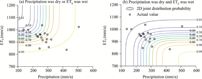
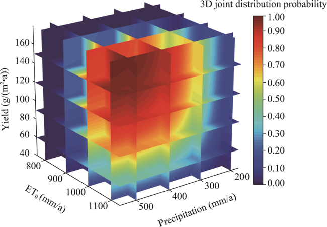
Drought, which restricts the sustainable development of agriculture, ecological health, and social economy, is affected by a variety of factors. It is widely accepted that a single variable cannot fully reflect the characteristics of drought events. Studying precipitation, reference evapotranspiration (ET0), and vegetation yield can derive information to help conserve water resources in grassland ecosystems in arid and semi-arid regions. In this study, the interactions of precipitation, ET0, and vegetation yield in Darhan Muminggan Joint Banner (DMJB), a desert steppe in Inner Mongolia Autonomous Region, China were explored using two-dimensional (2D) and three-dimensional (3D) joint distribution models. Three types of Copula functions were applied to quantitatively analyze the joint distribution probability of different combinations of precipitation, ET0, and vegetation yield. For the precipitation-ET0 dry-wet type, the 2D joint distribution probability with precipitation≤245.69 mm/a or ET0≥959.20 mm/a in DMJB was approximately 0.60, while the joint distribution probability with precipitation≤245.69 mm/a and ET0≥959.20 mm/a was approximately 0.20. Correspondingly, the joint return period that at least one of the two events (precipitation was dry or ET0 was wet) occurred was 2 a, and the co-occurrence return period that both events (precipitation was dry and ET0 was wet) occurred was 5 a. Under this condition, the interval between dry and wet events would be short, the water supply and demand were unbalanced, and the water demand of vegetation would not be met. In addition, when precipitation remained stable and ET0 increased, the 3D joint distribution probability that vegetation yield would decrease due to water shortage in the precipitation-ET0 dry-wet years could reach up to 0.60-0.70. In future work, irrigation activities and water allocation criteria need to be implemented to increase vegetation yield and the safety of water resources in the desert steppe of Inner Mongolia.

Cite this article

LI Hongfang , WANG Jian , LIU Hu , MIAO Henglu , LIU Jianfeng . Responses of vegetation yield to precipitation and reference evapotranspiration in a desert steppe in Inner Mongolia, China[J]. Journal of Arid Land, 2023 , 15(4) : 477 -490 . DOI: 10.1007/s40333-023-0051-2

1 Introduction

Grassland is an important part of terrestrial ecosystems and plays an important role in regulating climate, conserving soil and water, improving soil quality, and maintaining biodiversity (Wang et al., 2022a). A desert steppe is the transition zone between grassland and desert, and it is the most severe type of desertification among all grasslands. The desert steppe in Inner Mongolia Autonomous Region of China accounts for approximately 18.00% of the country's total grassland area (Li et al., 2013; Chu et al., 2014; Fang et al., 2016). The ecological environment of the desert steppe is fragile and extremely sensitive to precipitation changes (Zhan et al., 2007; Guo et al., 2012; Song et al., 2017; Legesse et al., 2022). Strong evaporation and surface radiation aggravate the water sensitivity of the desert steppe vegetation (Bittelli et al., 2008; Jung et al., 2010; Armstrong et al., 2015).
Precipitation and reference evapotranspiration (ET0) are two important, correlated random hydrological variables that characterize the relationship between regional water supply and plant demand (Li et al., 2017). At the same time, water is the main limiting factor affecting grassland ecosystems, which has been confirmed by controlled experiments and precipitation-gradient experiments (Bai et al., 2008; Yuan and Chen, 2009; Beier et al., 2012). In the desert steppe, monthly precipitation from May to August is decisive for annual precipitation. A study of the Inner Mongolia desert steppe reported that ET0 was between 570.00 and 1674.00 mm/a for the period from 1961 to 2010, and it was highest in western Inner Mongolia (Wang et al., 2015). The aridity of the arid region is expected to increase in the 21st century (Andrés et al., 2017). Studying the response characteristics of vegetation yield (hereinafter abbreviated as yield) in the desert steppe to precipitation and ET0 can not only reveal the quantitative risk of decreased yield because of water shortage under natural precipitation conditions, but also contribute to the understanding of ecological stability and yield security in the Inner Mongolia desert steppe.
Many studies on arid and semi-arid ecosystems analyzed single precipitation event, or revealed the changes of a certain factor with respect to precipitation change (Yan et al., 2018; Yu et al., 2019; Du et al., 2020). However, few researches have focused on the responses of yield to precipitation and ET0 in the desert steppe. Moreover, it is also difficult to quantitatively analyze the multivariate distribution probability of these variables. Thus, to more accurately predict the influence of precipitation on yield, it is necessary to understand how yield responds to precipitation and ET0 events. Copula functions are mathematical tools for solving multivariate probability problems and can reflect correlations between variables that are independent of the marginal distribution of random variables (Amirataee et al., 2020). Copula functions cannot limit the marginal distribution of variables. During the conversion process of the variables, the information of the original random variables will not change, especially when the variable dimension change is less than three. The multivariate probability model constructed from the Copula functions is simple and easy to apply (Xie et al., 2012). To date, Copula functions have been used extensively in hydrology-climate-related studies (e.g., Hao and Singh, 2015; Xu et al., 2015; Zhang et al., 2015; Cai et al., 2021). Copula fitting was used to analyze the distribution, duration, and intensity of droughts (e.g., Amirataee et al., 2020). For example, Wu et al. (2015) used a Copula function to study the variations in hydrological drought frequency in southern China. Additionally, the drought risk can be qualitatively described and quantitatively evaluated through different combinations of precipitation and ET0, thereby improving irrigation planning and scientific deployment of water resources (e.g., Vo et al., 2020).
To sum up, the three objectives of this study were as follows: (1) to obtain ET0 using the Penman-Monteith formula, and choose and verify a suitable marginal distribution and a Copula function for precipitation, ET0, and yield of the desert steppe in Inner Mongolia; (2) to use a Copula function to quantitatively evaluate the two-dimensional (2D) and three-dimensional (3D) joint distribution probability of precipitation, ET0, and yield in the desert steppe; and (3) to explore the main factors that influenced the yield of the desert steppe, and provide measures to mitigate desertification and improve sustainable vegetation development in this region.

2 Materials and methods

2.1 Study area

The study area is located in Darhan Muminggan Joint Banner (DMJB; 109°16′-111°25′E, 41°20′-42°40′N), a typical desert steppe with an area of approximately 1.81×10⁵ km2 in the central and western part of Inner Mongolia Autonomous Region, China. The area is a hilly desert steppe at the northern foot of Yinshan Mountain, and it is characterized by a temperate and semi-arid continental climate. The average annual precipitation is 253.45 mm, the annual average temperature is 4.12°C, and the average annual evaporation is 2480.57 mm (Song et al., 2017). The soil is dominated by brown soil and the vegetation is mainly perennial xerophytes. Species such as Artemisia frigida, Stipa krylovii, Stipa klemenzii, Stipa breviflora, and Cleistogenes songorica are the dominate plant species. The average vegetation coverage was 35.00% during 2002-2020. Data about the vegetation for this study were collected from the Yinshanbeilu Grassland Eco-hydrology National Observation and Research Station in DMJB (Fig. 1).
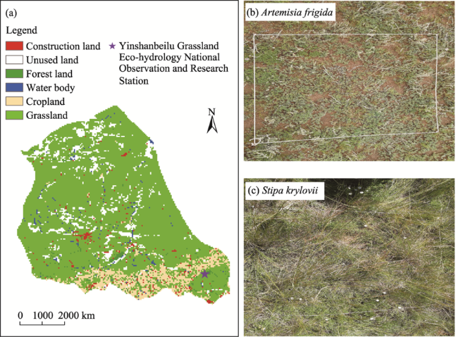
Fig. 1 Overview of land use/land cover in the study area (Darhan Muminggan Joint Banner; a), and photos showing Artemisia frigida (b) and Stipa krylovii (c)

2.2 Data sources

In this study, we collected daily meteorological data during 2002-2020 and annual data of yield in the main growing season (May-September) of 2002-2020. The daily precipitation, maximum temperature, minimum temperature, relative humidity, sunshine hours, solar radiation, water vapor pressure, and average wind speed data were provided by the China Meteorological Administration (http://cdc.cma.gov.cn). The data were collected and processed in accordance with the guide to the Global Observing System of the World Meteorological Organization and the technical specifications and standards for the weather observations of the China Meteorological Administration. The data of sunshine hours during July-December in 2020 were estimated from the average daily data of 2000-2019. The yield data of 2002-2020 were collected from an intensive pastoral region that covers an area of 1.33 km2. Artemisia frigida and Stipa krylovii were chosen as representative plant species to simulate yield in this study, as they dominated the composition of the plant community in the sampling plots and represented different functional groups (Zhao et al., 2006; Chen et al., 2013). In approximately mid-August every year (harvesting time), 5-10 plots (area of 1 m×1 m for each plot) with Artemisia frigida and Stipa krylovii as the dominant species were selected to survey, grid sample, measure, and evaluate for yield. One sample was taken from one plot. From 2002 to 2020, a total of 167 grass samples were collected, and the dry weight of the aboveground part was measured. The data statistics and analysis were performed using R (Lucent Technologies, New Jersey, USA) and Excel software. The graphics were preprocessed by MATLAB R2018b software (MathWorks, Massachusetts, USA). The time ranges of the data for this study are shown in Table 1.
Table 1 Description of the data used in this study
Type Factor Unit Period
Meteorological data Solar radiation kJ/(m2•d) 2002-2020
Minimum temperature °C 2002-2020
Maximum temperature °C 2002-2020
Relative humidity % 2002-2020
Water vapor pressure kPa 2002-2020
Average wind speed m/s 2002-2020
Precipitation mm/a 2002-2020
Sunshine hours h/d 2000-2019
Yield data Annual dry weight of yield per unit area g/(m2•a) 2002-2020

Note: Yield, vegetation yield.

2.3 Methods

2.3.1 Calculation of ET0

The Penman-Monteith formula was recommended by the United Nations Food and Agriculture Organization (FAO) in 1998 (Allen, 2000). It integrates data for elevation, latitude, wind speed, altitude, daily maximum temperature, daily minimum temperature, daily average temperature, daily average wind speed, daily average relative humidity, sunshine hours, and others. Then, ET0 is calculated as follows (Zhang et al., 2012):
$\mathop{\text{ET}}_{0}=\frac{0.408\Delta (Rn-G)+\gamma \frac{900u2(es-ea)}{T+273}}{\Delta +\gamma (1+0.34\mathop{u}_{2})},$
where ET0 is the reference evapotranspiration (mm/d); ∆ is the slope of the saturated vapor pressure-temperature curve (kPa/°C); Rn is the net solar radiation of the plant canopy surface (MJ/(m2•d)); G is the soil heat flux (MJ/(m2•d)), and the daily G was calculated in this study (G=0); γ is the hygrometer constant (kPa/°C); u2 is the wind speed at a height of 2 m (m/s); es and ea are the saturated water vapor pressure (kPa) and the actual water vapor pressure (kPa), respectively; and T is the average temperature (°C).

2.3.2 Marginal distribution

The Weibull (WEI), gamma (GAMMA), and Exponential (EXP) distributions were used to fit the marginal distributions of precipitation, ET0, and yield. The maximum likelihood method was applied to estimate the Copula function parameters, and then the Kolmogorov-Smirnov test (K-S test) was used to select the optimal marginal distribution (Song and Singh, 2010; Mohammadpour et al., 2012).
The WEI distribution function is given by:
$f(x)=\frac{b}{a}{{\left( \frac{x}{a} \right)}^{b-1}}\exp \left( -\frac{{{x}^{b}}}{a} \right),$
where f(x) is the marginal distribution function of x, where x is one of the variables (precipitation, ET0, or yield); a is the scale parameter; and b is the shape parameter.
The GAMMA distribution function is given by:
$f(x)=\frac{1}{\mathop{a}^{b}\text{ }\Gamma (b)}\mathop{x}^{b-1}\exp \left( -\frac{x}{a} \right),$
where Γ denotes the GAMMA function.
The EXP distribution function is given by:
$f(x)=\lambda \exp (-\lambda x),$
where λ is the scale parameter (λ>0).

2.3.3 Joint distribution model

A Copula function does not limit the marginal distribution of variables. With the Copula model, several arbitrary marginal distributions can be connected to form a multivariate joint distribution probability model. Copula functions are based on the Sklar's theorem (Sklar, 1959). Random variables (X1, X2, …, Xn (where n=3 in this study)) are continuous, and F1(X1), F2(X2),..., Fn(Xn) (where F is the n-dimensional joint probability distribution function) are their marginal distribution functions. Then, there exists a Copula function (C) such that:
$F({{X}_{1}},\text{ }{{X}_{2}},\text{ }...,\text{ }{{X}_{n}})=C\left[ {{F}_{1}}({{X}_{1}}),\text{ }{{F}_{2}}({{X}_{2}}),\text{ }...,\text{ }{{F}_{n}}({{X}_{n}}) \right].$
The K-S test statistic (D) that was used to select the optimal marginal distribution is defined as follows:
$D=\max _{1 \leq k \leq l}\left\{\left|c_k-\frac{m_k}{l}\right|,\left|c_k-\frac{m_k-1}{l}\right|\right\}$,
where ck is the Copula value of the joint observation sample (xk, yk) and mk is the number of joint observations that meet the conditions of x≤xk and y≤yk in the joint observation sample; k is the kth number; and l is the total number (l=19 in this study).
The Copula function is unique if the marginal distribution functions (F1(x1), F2(x2), …, Fn(xn)) are continuous. In this study, three commonly used functions, i.e., the Clayton Copula, Gumbel-Hougaard Copula, and Frank Copula functions (Lazoglou and Anagnostopoulou, 2019), were used to construct the 2D and 3D joint distributions of precipitation, ET0, and yield (Tables 2 and 3).
Table 2 Description of the two-dimensional (2D) Copula functions
Copula function Function expression Condition
Clayton $H(u,v)=\mathop{\left( \mathop{u}^{-\theta }+\mathop{v}^{-\theta }-1 \right)}^{-\text{ }\frac{1}{\theta }}$ θ≥0
Gumbel-Hougaard $H(u,v)=\exp \left\{ -\mathop{\left[ \mathop{(-\ln u)}^{\theta }+\mathop{(-\ln v)}^{\theta } \right]}^{-\text{ }\frac{1}{\theta }} \right\}$ θ≥1
Frank $H(u,v)=-\frac{1}{\theta }\ln \left[ 1+\frac{\left( \mathop{\text{e}}^{-\theta u}-1 \right)\left( \mathop{\text{e}}^{-\theta v}-1 \right)}{\mathop{\text{e}}^{-\theta }-1} \right]$ θ≠0

Note: The u and v are the marginal distribution functions of any two of precipitation, reference evapotranspiration (ET0), and yield; H(u, v) represents the joint distribution probability when both precipitation≤u (or ET0u or yield≤u) and precipitation≤v (or ET0v or yield≤v) occur; and θ is the Copula function parameter.

Table 3 Description of the three-dimensional (3D) Copula functions
Copula function Function expression Condition
Clayton $H({{u}_{1}},{{u}_{2}},{{u}_{3}})={{\left( {{u}_{1}}^{-\theta }+{{u}_{2}}^{-\theta }+{{u}_{3}}^{-\theta }-2 \right)}^{-\text{ }\frac{1}{\theta }}}$ θ≥0
Gumbel-Hougaard $H({{u}_{1}},{{u}_{2}},{{u}_{3}})=\exp \left\{ -\left[ {{(-\ln {{u}_{1}})}^{\theta }}+{{(-\ln {{u}_{2}})}^{\theta }}+{{(-\ln {{u}_{3}})}^{\theta }} \right] \right.\left. ^{-\text{ }\frac{1}{\theta }} \right\}$ θ≥1
Frank $H({{u}_{1}},{{u}_{2}},{{u}_{3}})=-\frac{1}{\theta }\ln \left[ 1+\frac{\left( {{\text{e}}^{-\theta {{u}_{1}}}}-1 \right)\left( {{\text{e}}^{-\theta {{u}_{2}}}}-1 \right)\left( {{\text{e}}^{-\theta {{u}_{3}}}}-1 \right)}{{{\left( {{\text{e}}^{-\theta }}-1 \right)}^{2}}} \right]$ θ>0

Note: The u1, u2, and u3 are the marginal distribution functions of precipitation, ET0, and yield, respectively; and H(u1, u2, u3) represents the joint distribution probability when precipitation≤u1, ET0u2, and yield≤u3 all occur.

The Copula function goodness-of-fit test is the premise for selecting the optimal Copula functions. Here, the fitting of the Copula functions was tested using the root mean square error (RMSE) and Akaike information criterion (AIC). The fitting test and the goodness-of-fit (Li et al., 2013), with the minimum AIC as the best fit criterion, were calculated as follows:
$\text{MSE}=\frac{1}{N-1}\sum\limits_{i=1}^{N}{{{({{P}_{ei}}-{{P}_{i}})}^{2}}}$,
$\text{RMSE}=\sqrt{\text{MSE}}$,
$\text{AIC}=N\ln \left( \text{MSE} \right)\text{+}2k$,
${{P}_{e}}({{x}_{i}},{{y}_{i}})=\frac{Num({{x}_{j}}\le {{x}_{i}},{{y}_{j}}\le {{y}_{i}})-0.44}{t+0.12},$
where MSE is the mean square error; N is the total number of joint observations; Pei is the empirical frequency; Pi is the theoretical frequency; RMSE is the root mean square error; Pe(xi, yi) is the empirical frequency of the 2D joint distribution; Num(xj≤xi, yj≤yi) indicates the number of joint observation value less than or equal to (xi, yi); and t is the number of observation value.
${{P}_{e}}({{x}_{i}},{{y}_{i}},{{z}_{i}})=\frac{Num({{x}_{j}}\le {{x}_{i}},{{y}_{j}}\le {{y}_{i}},{{z}_{j}}\le {{z}_{i}})-0.44}{t+0.12},$
where Pe(xi, yi, zi) is the empirical frequency of the 3D joint distribution and Num(xj≤xi, yj≤yi, zj≤zi) indicates the number of joint observation value less than or equal to (xi, yi, zi).

2.3.4 Joint distribution probability and return period

Using the pf(wet) and pk(dry) (where pf and pk are the frequency values for dividing the annual precipitation or ET0 into wet and dry, respectively) of 37.50% and 62.50%, respectively, as the frequency values for dividing the annual precipitation or ET0 into wet, normal, and dry, we analyzed the interannual differences among them with the 2D Copula joint distribution model (Yan et al., 2007). We further determined the occurrences of wet, normal, and dry seasons, which can be divided into nine situations (Yan et al., 2007), as shown in Table 4.
Table 4 Division of occurrences of wet, normal, and dry situations for precipitation-ET0
Situation Frequency
Precipitation-ET0 wet-wet type ${{p}_{1}}=p(X\ge {{x}_{pf}},\text{ }Y\ge {{y}_{pf}})$
Precipitation-ET0 wet-normal type ${{p}_{2}}=p(X\ge {{x}_{pf}},\text{ }{{y}_{pf}}<Y<{{y}_{pf}})$
Precipitation-ET0 wet-dry type ${{p}_{3}}=p(X\ge {{x}_{pf}},\text{ }Y\le {{y}_{pk}})$
Precipitation-ET0 normal-wet type ${{p}_{4}}=p({{x}_{pk}}<X<{{x}_{pf}},\text{ }Y\ge {{y}_{pf}})$
Precipitation-ET0 normal-normal type ${{p}_{5}}=p({{x}_{pk}}<X<{{x}_{pf}},\text{ }{{y}_{pk}}<Y<{{y}_{pf}})$
Precipitation-ET0 normal-dry type ${{p}_{6}}=p({{x}_{pk}}<X<{{x}_{pf}},\text{ }Y\le {{y}_{pk}})$
Precipitation-ET0 dry-wet type ${{p}_{7}}=p(X\le {{x}_{pk}},\text{ }Y\ge {{y}_{pf}})$
Precipitation-ET0 dry-normal type ${{p}_{8}}=p(X\le {{x}_{pk}},\text{ }{{y}_{pk}}<Y\le {{y}_{pf}})$
Precipitation-ET0 dry-dry type ${{p}_{9}}=p(X\le {{x}_{pk}},\text{ }Y\le {{y}_{pk}})$

Note: ET0, reference evapotranspiration; p1-p9, the frequency of nine situations; X, the series of precipitation; Y, the series of (ET0); pf and pk, the frequency values for dividing precipitation or ET0 into wet and dry, respectively; xpf and xpk, the values for dividing precipitation into wet and dry, respectively; ypf and ypk, the values for dividing ET0 into wet and dry, respectively.

Given that the main aim of this study was to evaluate the risk of decreased yield under the wet, normal, or dry condition of the Inner Mongolia desert steppe, we focused on the two joint distribution probabilities of the precipitation-ET0 dry-wet type and their return periods:
$\left\{ \begin{matrix} {{G}_{X,\text{ }Y}}(x,y)=P(X\le x \text{or} Y\ge y)=1-{{F}_{Y}}(y)+F(x,y) \\ G_{X,\text{ }Y}^{\prime }(x,y)=P(X\le x,Y\ge y)={{F}_{X}}(x)-F(x,y) \\\end{matrix} \right.,$
$\left\{\begin{array}{l}T_{x,y}=\dfrac{1}{G_{X,Y}(x,y)}\\ T_{X,y}'=\dfrac{1}{ G_{X,Y}'(x,y)}\end{array}\right.,$
where GX, Y(x, y) and P(X≤x or Y≥y) refer to the joint distribution probability when at least one of the two events that X does not exceed a certain value or Y exceeds a certain value occurs; G'X, Y(x, y) and P(X≤x, Y≥y) refer to the joint distribution probability when two events that X does not exceed a certain value and Y exceeds a certain value occur; FX(x) and FY(y) are the marginal distributions of precipitation and ET0; F(x, y) is the joint probability distribution function of X≤x and Y≤y; Tx, y is the joint return period; and T'x, y indicates the co-occurrence return period in which the two events occur simultaneously.

3 Results

3.1 Marginal distributions of precipitation, ET0, and yield, and division of precipitation and ET0

The series of precipitation, ET0, and yield in DMJB from 2002 to 2020 are shown in Figure 2. ET0 in DMJB was generally negatively correlated with precipitation and yield, while precipitation and yield were positively correlated with each other. The difference between precipitation and ET0 fluctuated in the range of approximately 400.00-900.00 mm/a during the study period and was greatest in 2009, at 863.66 mm/a.
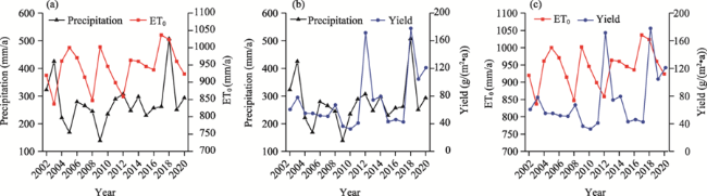
Fig. 2 Relationships between precipitation and reference evapotranspiration (ET0; a), precipitation and yield (vegetation yield; b), and ET0 and yield (c) from 2002 to 2020
With a significance level of α=0.05, precipitation, ET0, and yield in DMJB conformed to the GAMMA distribution (Table 5), which is a special form of Pearson type III distribution. When the significance level of the K-S test was 0.05 (n=19), the corresponding quantile was 0.30. The K-S test statistics that corresponded to precipitation, ET0, and yield for the GAMMA distribution were 0.16, 0.11, and 0.17, respectively, which were all less than the corresponding quantile values, and the corresponding P values were all greater than 0.05. This indicates that the GAMMA distribution was appropriate and could provide values for dividing precipitation and ET0 to wet, normal, and dry conditions in DMJB (Table 6).
Table 5 Parameters of the univariate marginal distributions
Characteristic variable Marginal distribution function Parameter K-S test
Shape Scale Statistic P
Precipitation WEI 3.45 304.7600 0.20 0.38
GAMMA 13.18 0.0500 0.16 0.68
EXP - 0.0036 0.45 0.04×10⁻²
ET0 WEI 19.99 967.4000 0.13 0.85
GAMMA 288.14 0.3100 0.11 0.95
EXP - 0.0011 0.59 8.59×10⁻⁷
Yield WEI 1.92 83.0500 0.19 0.45
GAMMA 4.11 0.0600 0.17 0.55
EXP - 0.0100 0.36 0.01

Note: WEI, Weibull; GAMMA, gamma; EXP, Exponential; K-S test, Kolmogorov-Smirnov test. K-S test statistic represents the maximum distance between the two distributions; the smaller the statistic, the smaller the gap between the two distributions and the more consistent the two distributions. The larger the P value, the more the null hypothesis cannot be rejected (P>0.05) and the more similarity between the two distributions. - indicates that there are no shape parameters.

Table 6 Division values for dividing precipitation and ET0 into wet and dry
Wet (frequency of 37.50%) Dry (frequency of 62.50%)
Precipitation (mm/a) ET0 (mm/a) Precipitation (mm/a) ET0 (mm/a)
Division value 293.38 959.20 245.69 923.84

3.2 Joint distributions of precipitation, ET0, and yield

The maximum likelihood method was used to calculate the Copula functions parameters. The RMSE between the empirical frequency and theoretical frequency was calculated by the Copula functions, and the minimum AIC was used as the criterion for selecting the optimal fitting functions. The corresponding results are shown in Table 7. Because precipitation and yield were negatively correlated with ET0, only the Frank Copula function was suitable as their joint function. Precipitation and yield were positively correlated with each other. For the relationship between precipitation and yield, the Gumbel-Hougaard Copula function had the smallest AIC and RMSE values and the best goodness-of-fit. For ET0 and yield, the Frank Copula function had the best goodness-of-fit, with AIC and RMSE values of -75.53 and 0.13, respectively.
Table 7 Parameter values and goodness-of-fit tests of the Copula functions
Relationship of variables Copula function θ AIC RMSE
Precipitation-ET0 Frank -2.71 -82.85 0.11
Precipitation-yield Frank 4.13 -62.95 0.18
Clayton 1.03 -90.30 0.09
Gumbel-Hougaard 1.84 -97.22 0.07
ET0-yield Frank -1.11 -115.79 0.05
Precipitation-ET0-yield Frank 0.09 -75.53 0.13
Clayton 0.24 -72.85 0.14
Gumbel-Hougaard 1.24 -69.86 0.15

Note: θ, Copula function parameter; AIC, Akaike information criterion; RMSE, root mean square error. The Copula function with the smallest AIC and RMSE values was selected as the most appropriate probability distribution.

As shown in Figure 3, the empirical frequency and theoretical frequency of the joint distributions of precipitation, ET0, and yield in DMJB based on the Copula functions were uniformly distributed around the 45° diagonal line, indicating that the obtained Copula functions fitted well. The goodness-of-fit was best for precipitation-yield (Fig. 3c) and ET0-yield (Fig. 3d), with the R2 values of 0.96 for both the empirical frequency and theoretical frequency, followed by precipitation-ET0 (Fig. 3b), with the R2 value of 0.88. However, the R2 value for the relationship of precipitation-ET0-yield, at 0.76, was the smallest (Fig. 3a). These results show that the selected Copula functions were reasonable.
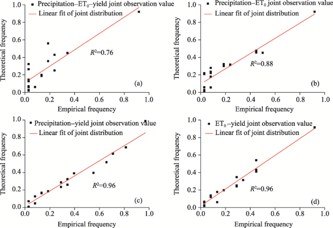
Fig. 3 Empirical frequency and theoretical frequency of joint distributions of precipitation-ET0-yield (a), precipitation-ET0 (b), precipitation-yield (c), and ET0-yield (d)

3.3 Joint distribution probability of precipitation, ET0, and yield

3.3.1 2D joint distribution probability

The 2D joint distribution probability contours of precipitation-ET0, precipitation-yield, and ET0-yield, and the distributions of the actual values of precipitation, ET0, and yield during 2002-2020 are plotted in Figure 4. The patterns in the trends of the 2D joint distribution probability values for precipitation-ET0, precipitation-yield, and ET0-yield were the same. The actual years for precipitation-ET0 joint distribution with precipitation≤300.00 mm/a and ET0≤1000.00 mm/a were 12 a in DMJB during 2002-2020, accounting for 63.16% of the total studied years, while the 2D joint distribution probability of precipitation-ET0 with precipitation≤300.00 mm/a and ET0≤1000.00 mm/a was 0.53 (Fig. 4a). The actual years for precipitation-yield joint distribution with precipitation≤300.00 mm/a and yield≤80.00 g/(m2•a) were 13 a, accounting for 68.42% of the total studied years, while the 2D joint distribution probability of precipitation-yield with precipitation≤300.00 mm/a and yield≤80.00 g/(m2•a) was approximately 0.53 (Fig. 4b). The actual years for precipitation-ET0 joint distribution with ET0≤1000.00 mm/a and yield≤80.00 g/(m2•a) were 13 a in DMJB during 2002-2020, mainly concentrated in 2002-2016, and the 2D joint distribution probability of precipitation-ET0 with ET0≤1000.00 mm/a and yield≤80.00 g/(m2•a) was approximately 0.53 (Fig. 4c). These results indicate that the ranges of the joint distributions of precipitation-ET0, precipitation-yield, and ET0-yield were relatively stable in DMJB during 2002-2020. The probability that yield would be ≤80.00 g/(m2•a) was approximately 0.50.
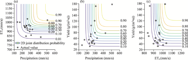
Fig. 4 Two dimensional (2D) joint distribution contours of precipitation-ET0 (a), precipitation-yield (b), and ET0-yield (c) in DMJB

3.3.2 Frequency analysis of the 2D joint distributions of the wet, normal, and dry conditions for precipitation-ET0

For the nine combinations of wet, normal, and dry conditions, the combination of the dry-wet type for precipitation-ET0 was the most unfavorable for irrigation scheduling. Figure 5 shows the 2D joint distribution contours of precipitation-ET0 and the distributions of the actual precipitation and ET0 values in DMJB during 2002-2020. Specifically, Figure 5a indicates the joint distribution probability that at least one of the two events occurred, i.e., precipitation was dry or ET0 was wet, and Figure 5b shows the joint distribution probability that both events occurred, i.e., precipitation was dry and ET0 was wet. Overall, the patterns of changes in the joint probability values were the same, and they all increased with the increase of precipitation and the decrease of ET0. The joint distribution probability for the precipitation-ET0 dry-wet type with the actual value of precipitation≤245.69 mm/a or ET0≥959.20 mm/a was approximately 0.60 during 2002-2020, and there were 12 a in this range, accounting for 63.16% of the total studied years. However, the joint distribution probability for the precipitation-ET0 dry-wet type with precipitation≤245.69 mm/a and ET0≥959.20 mm/a was approximately 0.20, and there were 3 a in this range, accounting for 15.79% of the total studied years.
Fig. 5 2D joint distribution probability contours of precipitation-ET0 with at least one of the two events (precipitation was dry or ET0 was wet) occurred (a) and with both events (precipitation was dry and ET0 was wet) occurred (b)
The joint return period that at least one of the two events (precipitation was dry or ET0 was wet) occurred was 2 a, and the co-occurrence return period that both events (precipitation was dry and ET0 was wet) occurred was 5 a. These values were calculated from Equation 11 and were based on the joint distribution probability of the precipitation-ET0 dry-wet type in DMJB. The water supply and demand imbalance of DMJB is more likely when there is natural precipitation. Under this condition, the interval between dry and wet events would be short, and the risk of vegetation water demand not being met is greater.

3.3.3 3D joint distribution probability

The analysis in Table 7 indicated that the Frank Copula function could be applied to the 3D joint distribution of precipitation, ET0, and yield when precipitation≤u1 (where u1 is the marginal distribution function of precipitation), ET0u2 (where u2 is the marginal distribution function of ET0), and yield≤u3 (where u3 is the marginal distribution function of yield) all occurred in DMJB. The 3D joint distribution probability of precipitation, ET0, and yield is shown in Figure 6. The average yield per unit area was 73.05 g/(m2•a) in DMJB during 2002-2020. When precipitation was dry and ET0 was wet, as in 2004, 2005, and 2009, the average yield per unit area was at a low level (48.74 g/(m2•a)), and the 3D joint distribution probability of precipitation-ET0-yield with precipitation≤245.69 mm/a, ET0≤959.20 mm/a, and yield≤48.74g/(m2•a) was 0.07. When precipitation was dry or ET0 was wet, the average yield per unit area was 68.24 g/(m2•a), and the 3D joint distribution probability of precipitation-ET0-yield with precipitation≤245.69 mm/a, ET0≤959.20 mm/a, and yield≤68.24 g/(m2•a) was 0.12. Of these, when precipitation was stable and ET0 increased, the 3D joint distribution probability that yield would decrease due to water shortage in a year with the precipitation-ET0 dry-wet type could reach 0.60-0.70. In addition, as shown in Figure 6, when ET0 was lower than 900.00 mm/a, the 3D joint distribution probability that yield would decrease was less than 0.30, indicating that the yield of the desert steppe was sensitive to precipitation and other factors such as temperature, wind speed, and sunshine hours.
Fig. 6 Three dimensional (3D) joint distribution probability of precipitation, ET0, and yield in DMJB

4 Discussion

During the crop growth period, precipitation and ET0 are the main factors that cause agricultural drought. Batsukh et al. (2021) used ET0 to predict the evapotranspiration of a specific biological community in the desert steppe of Inner Mongolia in the absence of meteorological data. Han et al. (2015) studied the temporal and spatial dynamics of climate and vegetation phenology in the desert steppe of Inner Mongolia and found that the primary productivity decreased from southeast to northwest along the precipitation gradient. Precipitation can affect vegetation growth when it is transformed into soil water through interception by the vegetation canopy (Sugita et al., 2015). However, the previous studies are relatively one dimensional and lack of multivariate research on the desert steppe (Zhu et al., 2022). The joint distribution probability for the precipitation-ET0 dry-wet type with the actual value of precipitation≤245.69 mm/a or ET0≥959.20 mm/a was approximately 0.60 during 2002-2020 in our study.
On the basis of previous research, we quantitatively analyzed and predicted the 2D and 3D joint risk probabilities of precipitation, ET0, and yield of the desert steppe in Inner Mongolia. The results show that for the precipitation-ET0 dry-wet type, the 2D joint distribution probability with the actual precipitation≤245.69 mm/a or ET0≥959.20 mm/a in DMJB was approximately 0.60, while the 2D joint distribution probability with precipitation≤245.69 mm/a and ET0≥959.20 mm/a was approximately 0.20. The joint return period and the co-occurrence return period were calculated as 2 and 5 a, respectively (Fig. 4), indicating that drought risk is higher in the precipitation-ET0 dry-wet years, which could increase the degradation of grasslands in Inner Mongolia (Hu et al., 2019). This result is consistent with the finding that evapotranspiration would further increase under the background of global warming (Li et al., 2016). The desert steppe was also affected by changes in ET0 (Figs. 3c and 6), which is consistent with the fact that ET0 in the temperate desert steppe of Inner Mongolia can be well estimated using only meteorological variables and the Penman-Monteith equation (Yang and Zhou, 2011). Previous studies also demonstrated that the effect of small precipitation events (0.00-5.00 mm) on plant assimilation was limited (e.g., Song et al., 2017). Our results showed that when ET0 was lower than 900.00 mm/a, the 3D joint distribution probability of decreased yield would be less than 0.30 (Fig. 6), suggesting that the yield of the desert steppe was sensitive to precipitation and other factors such as temperature, wind speed, and sunshine hours (Wang et al., 2022b). Therefore, artificial precipitation, reduction of grazing, and other measures are needed in years with the precipitation-ET0 dry-wet type to ensure the sustainable development of the desert steppe, and adaptability to drought is also essential for the growth of grassland species.
This study plays an important role in analyzing the probability of dry and wet events during the crop growth periods in the desert steppe of Inner Mongolia and guiding agricultural drought control. However, there were some limitations in data processing in our work. The vegetation data were limited. As Artemisia frigida and Stipa krylovii are the dominant plant species in DMJB, rare varieties were ignored in vegetation collection. In addition, although the suitable Copula functions selected by the marginal distributions of precipitation, ET0, and yield had a good fit (Fig. 3; Table 7), there were certain deviations in the software precision. In the future, related studies on the desert steppe should consider other factors, such as biodiversity. It is also worth exploring the feedback mechanisms between soil organisms and hydrological cycle in arid and semi-arid regions.

5 Conclusions

This study focused on the response of yield to precipitation and ET0 in wet and dry years in a typical desert steppe (DMJB) in Inner Mongolia. We also examined how precipitation, ET0, and yield interacted in DMJB during 2002-2020. The three variables all obeyed the GAMMA distribution, and the joint distribution models of precipitation-ET0-yield, precipitation-ET0, and ET0-yield established by the Frank Copula function fitted well. The Gumbel-Hougaard Copula function exhibited the best fit for the joint distribution model of precipitation-yield. The R2 values of the empirical frequency and theoretical frequency were all higher than 0.70, and the 3D joint distribution probability of precipitation-ET0-yield with precipitation≤245.69 mm/a, ET0≤959.20 mm/a, and yield≤48.74g/(m2•a) was 0.07. The joint distribution probability values of precipitation and ET0 all increased with the increase of precipitation and the decrease of ET0 in DMJB. Under natural precipitation, there was a relatively high risk in DMJB that the water supply would not meet the water demand of the vegetation, and the interval time between dry and wet events was short. For the precipitation-ET0 dry-wet type, the 2D joint distribution probability with precipitation≤245.69 mm/a or ET0≥959.20 mm/a in DMJB was approximately 0.60, while the joint distribution probability with precipitation≤245.69 mm/a and ET0≥959.20 mm/a was approximately 0.20. Further, the joint return period and the co-occurrence return period were 2 and 5 a, respectively. Irrigation activities and water allocation criteria need to be implemented to ensure the success of agriculture and animal husbandry in the precipitation-ET0 dry-wet years.
In the future, the research scope can be expanded to the whole Inner Mongolia grassland, then the location-varied patterns can be deduced through the spatial variations, and the joint distributions of precipitation, ET0, and yield can be analyzed at different locations.

Acknowledgements

This research was supported by the Natural Science Foundation of Inner Mongolia Autonomous Region, China (2022QN04003) and the Central Government to Guide Local Scientific and Technological Development (2021ZY0031).
[1]
Allen R G. 2000. Using the FAO-56 dual crop coefficient method over an irrigated region as part of an evapotranspiration intercomparison study. Journal of Hydrology, 229(1-2): 27-41.

[2]
Amirataee B, Montaseri M, Rezaie H. 2020. An advanced data collection procedure in bivariate drought frequency analysis. Hydrological Processes, 34(21): 4067-4082.

[3]
Andrés P, Moore J C, Cotrufo F, et al. 2017. Grazing and edaphic properties mediate soil biotic response to altered precipitation patterns in a semiarid prairie. Soil Biology and Biochemistry, 113: 263-274.

[4]
Armstrong R N, Pomeroy J W, Martz L W. 2015. Variability in evaporation across the Canadian Prairie region during drought and non-drought periods. Journal of Hydrology, 521: 182-195.

[5]
Bai Y F, Wu J G, Xing Q, et al. 2008. Primary production and rain use efficiency across a precipitation gradient on the Mongolia Plateau. Ecology, 89(8): 2140-2153.

[6]
Batsukh K, Zlotnik V A, Suyker A, et al. 2021. Prediction of biome-specific potential evapotranspiration in Mongolia under a scarcity of weather data. Water, 13(18): 2470, doi: 10.3390/w13182470.

[7]
Beier C, Beierkuhnlein C, Wohlgemuth T, et al. 2012. Precipitation manipulation experiments-challenges and recommendations for the future. Ecology Letter, 15(8): 899-911.

[8]
Bittelli M, Ventura F, Campbell G S, et al. 2008. Coupling of heat, water vapor, and liquid water fluxes to compute evaporation in bare soils. Journal of Hydrology, 362(3-4): 191-205.

[9]
Cai S H, Song X N, Hu R H, et al. 2021. Spatiotemporal characteristics of agricultural droughts based on soil moisture data in Inner Mongolia from 1981 to 2019. Journal of Hydrology, 603: 127104, doi: 10.1016/j.jhydrol.2021.127104.

[10]
Chen L P, Zhao N X, Zhang L H, et al. 2013. Responses of two dominant plant species to drought stress and defoliation in the Inner Mongolia Steppe of China. Plant Ecology, 214(2): 221-229.

[11]
Chu C, Havstad K M, Kaplan N, et al. 2014. Life form influences survivorship patterns for 109 herbaceous perennials from six semi-arid ecosystems. Journal of Vegetation Science, 25(4): 947-954.

[12]
Du N, Li W, Qiu L, et al. 2020. Mass loss and nutrient release during the decomposition of sixteen types of plant litter with contrasting quality under three precipitation regimes. Ecology and Evolution, 10(7): 3367-3382.

[13]
Fang J Y, Bai Y F, Li L H, et al. 2016. Scientific basis and practical ways for sustainable development of China's pasture regions. Chinese Science Bulletin, 61(2): 155-164.

[14]
Guo Q, Hu Z M, Li S G, et al. 2012. Spatial variations in aboveground net primary productivity along a climate gradient in Eurasian temperate grassland: Effects of mean annual precipitation and its seasonal distribution. Global Change Biology, 18(12): 3624-3631.

[15]
Han F, Zhang Q, Buyantuev A, et al. 2015. Effects of climate change on phenology and primary productivity in the desert steppe of Inner Mongolia. Journal of Arid Land, 7(2): 251-263.

[16]
Hao Z C, Singh V P. 2015. Drought characterization from a multivariate perspective: A review. Journal of Hydrology, 527: 668-678.

[17]
Hu X X, Mitsuru H, Wu Y N, et al. 2019. Responses in gross primary production of Stipa krylovii and Allium polyrhizum to a temporal rainfall in a temperate grassland of Inner Mongolia, China. Journal of Arid Land, 11(6): 824-836.

[18]
Jung M, Reichstein M, Ciais P, et al. 2010. Recent decline in the global land evapotranspiration trend due to limited moisture supply. Nature, 467: 951-954.

[19]
Lazoglou G, Anagnostopoulou C. 2019. Joint distribution of temperature and precipitation in the Mediterranean, using the Copula method. Theoretical and Applied Climatology, 135(3-4): 1399-1411.

[20]
Legesse T G, Qu L P, Dong G, et al. 2022. Extreme wet precipitation and mowing stimulate soil respiration in the Eurasian meadow steppe. Science of the Total Environment, 851(1): 158130, doi: 10.1016/j.scitotenv.2022.158130.

[21]
Li C, Singh V P, Mishra A K. 2013. A bivariate mixed distribution with a heavy-tailed component and its application to single-site daily rainfall simulation. Water Resources Research, 49(2): 767-789.

[22]
Li F, Zhao W Z, Liu H. 2013. The response of aboveground net primary productivity of desert vegetation to rainfall pulse in the temperate desert region of northwest China. PLoS ONE, 8(9): e73003, doi: 10.1371/journal.pone.0073003.

[23]
Li H D, Wang A Z, Yuan F H, et al. 2016. Evapotranspiration dynamics over a temperate meadow ecosystem in eastern Inner Mongolia, China. Environmental Earth Sciences, 75: 978, doi: 10.1007/s12665-016-5786-z.

[24]
Li M, Fu Q, Singh V P, et al. 2017. An intuitionistic fuzzy multi-objective non-linear programming model for sustainable irrigation water allocation under the combination of dry and wet conditions. Journal of Hydrology, 555: 80-84.

[25]
Mohammadpour O, Hassanzadeh Y, Khodadadi A, et al. 2012. Probabilistic risk analysis of flood events using trivariate copulas. Theoretical and Applied Climatology, 111: 341-360.

[26]
Sala O E, Lauenroth W K. 1982. Small rainfall events: An ecological role in semiarid regions. Oecologia, 53(3): 301-304.

[27]
Sklar A. 1959. Dimension distribution functions and their margins. Statistical Institute of the University of Paris, 8: 229-231. (in French)

[28]
Song S, Singh V P. 2010. Frequency analysis of droughts using the Plackett copula and parameter estimation by genetic algorithm. Stochastic Environmental Research & Risk Assessment, 24(5): 783-805.

[29]
Song Y F, Guo Z X, Lu Y J, et al. 2017. Pixel-level spatiotemporal analyses of vegetation fractional coverage variation and its influential factors in a desert steppe: A case study in Inner Mongolia, China. Water, 9(7): 478, doi: 10.3390/w9070478.

[30]
Sugita M, Yoshizawa S, Byambakhuu I. 2015. Limiting factors for nomadic pastoralism in Mongolian steppe: A hydrologic perspective. Journal of Hydrology, 524: 455-467.

[31]
Vo Q T, So J M, Bae D H. 2020. An integrated framework for extreme drought assessments using the natural drought index, Copula and Gi* Statistic. Water Resources Management, 34(3): 1353-1368.

[32]
Wang S N, Li R P, Wu Y J, et al. 2022a. Vegetation dynamics and their response to hydrothermal conditions in Inner Mongolia, China. Global Ecology and Conservation, 34: e02034, doi: 10.1016/j.gecco.2022.e02034.

[33]
Wang S N, Li R P, Wu Y J, et al. 2022b. Effects of multi-temporal scale drought on vegetation dynamics in Inner Mongolia from 1982 to 2015, China. Ecological Indicators, 136: 108666, doi: 10.1016/j.ecolind.2022.108666.

[34]
Wang X X, Pan X B, Gu S H, et al. 2015. Trend in reference crop evapotranspiration and meteorological factors affecting trends in Inner Mongolia. Transactions of the Chinese Society of Agricultural Engineering, 31(1): 142-152. (in Chinese)

[35]
Wu Z, Lin Q, Lu G, et al. 2015. Analysis of hydrological drought frequency for the Xijiang River Basin in South China using observed streamflow data. Natural Hazards, 77(3): 1655-1677.

[36]
Xie H, Luo Q, Huang J. 2012. Synchronous asynchronous encounter analysis of multiple hydrologic regions based on 3D copula function. Advances in Water Science, 23(2): 186-193. (in Chinese)

[37]
Xu K, Yang D, Xu X, et al. 2015. Copula based drought frequency analysis considering the spatio-temporal variability in Southwest China. Journal of Hydrology, 527: 630-640.

[38]
Yan B W, Guo S L, Xiao Y. 2007. Synchronous-asynchronous encounter probability of rich-poor precipitation between water source area and water receiving areas in the Middle Route of South-to-North Water Transfer Project. Journal of Hydraulic Engineering, 38(10): 1178-1185. (in Chinese)

[39]
Yan Z Q, Qi Y C, Dong Y S, et al. 2018. Precipitation and nitrogen deposition alter litter decomposition dynamics in semiarid temperate steppe in Inner Mongolia, China. Rangeland Ecology and Management, 71(2): 220-227.

[40]
Yang F L, Zhou G S. 2011. Characteristics and modeling of evapotranspiration over a temperate desert steppe in Inner Mongolia, China. Journal of Hydrology, 396(1-2): 139-147.

[41]
Yu S Q, Mo Q F, Li Y W, et al. 2019. Changes in seasonal precipitation distribution but not annual amount affect litter decomposition in a secondary tropical forest. Ecology and Evolution, 9(19): 11344-11352.

[42]
Yuan Z Y, Chen H. 2009. Global scale patterns of nutrient resorption associated with latitude, temperature and precipitation. Global Ecology and Biogeography, 18(1): 11-18.

[43]
Zhan X, Li L, Cheng W. 2007. Restoration of Stipa krylovii steppes in Inner Mongolia of China: Assessment of seed banks and vegetation composition. Journal of Arid Environments, 68(2): 298-307.

[44]
Zhang F, Zhou G, Wang Y, et al. 2012. Evapotranspiration and crop coefficient for a temperate desert steppe ecosystem using eddy covariance in Inner Mongolia, China. Hydrological Processes, 26(3): 379-386.

[45]
Zhang Q, Xiao M, Singh V P. 2015. Uncertainty evaluation of copula analysis of hydrological droughts in the East River basin, China. Global & Planetary Change, 129(7): 1-9.

[46]
Zhao N X, Gao Y B, Wang J L, et al. 2006. Genetic diversity and population differentiation of the dominant species Stipa krylovii in the Inner Mongolia steppe. Biochemical Genetics, 44(11-12): 513-526.

[47]
Zhu Y, Yu K L, Wu Q, et al. 2022. Seasonal precipitation and soil microbial community influence plant growth response to warming and N addition in a desert steppe. Plant and Soil, 258: 1-15.

Outlines

/