Research article

Future meteorological drought conditions in southwestern Iran based on the NEX-GDDP climate dataset

  • Sakine KOOHI ,
  • Hadi RAMEZANI ETEDALI , *
Expand
  • Department of Water Engineering, Faculty of Agriculture and Natural Resources, Imam Khomeini International University, Qazvin 96818, Iran
*Hadi RAMEZANI ETEDALI (E-mail: )

Received date: 2022-03-04

  Revised date: 2022-06-02

  Accepted date: 2022-06-28

  Online published: 2023-04-30

Abstract

Investigation of the climate change effects on drought is required to develop management strategies for minimizing adverse social and economic impacts. Therefore, studying the future meteorological drought conditions at a local scale is vital. In this study, we assessed the efficiency of seven downscaled Global Climate Models (GCMs) provided by the NASA Earth Exchange Global Daily Downscaled Projections (NEX-GDDP), and investigated the impacts of climate change on future meteorological drought using Standard Precipitation Index (SPI) in the Karoun River Basin (KRB) of southwestern Iran under two Representative Concentration Pathway (RCP) emission scenarios, i.e., RCP4.5 and RCP8.5. The results demonstrated that SPI estimated based on the Meteorological Research Institute Coupled Global Climate Model version 3 (MRI-CGCM3) is consistent with the one estimated by synoptic stations during the historical period (1990-2005). The root mean square error (RMSE) value is less than 0.75 in 77% of the synoptic stations. GCMs have high uncertainty in most synoptic stations except those located in the plain. Using the average of a few GCMs to improve performance and reduce uncertainty is suggested by the results. The results revealed that with the areas affected by wetness decreasing in the KRB, drought frequency in the North KRB is likely to increase at the end of the 21st century under RCP4.5 and RCP8.5 scenarios. At the seasonal scale, the decreasing trend for SPI in spring, summer, and winter shows a drought tendency in this region. The climate-induced drought hazard can have vast consequences, especially in agriculture and rural livelihoods. Accordingly, an increasing trend in drought during the growing seasons under RCP scenarios is vital for water managers and farmers to adopt strategies to reduce the damages. The results of this study are of great value for formulating sustainable water resources management plans affected by climate change.

Cite this article

Sakine KOOHI , Hadi RAMEZANI ETEDALI . Future meteorological drought conditions in southwestern Iran based on the NEX-GDDP climate dataset[J]. Journal of Arid Land, 2023 , 15(4) : 377 -392 . DOI: 10.1007/s40333-023-0097-1

1 Introduction

Drought is one of the natural hazards that can affect numerous sectors, such as agriculture, water resources, environment, society, and ecosystem, which is related to global and regional food security (Wilhite, 2000; Ionita et al., 2016; Aziz et al., 2018; Modarresi Rad et al., 2021). Changes in precipitation and meteorological parameters are the first consequences of drought that lead to river flow changes. Next, it can be seen that the shortage of water resources affects agricultural activities. As a result, social and economic effects and consequences appear (Adamson and Bird, 2010). Therefore, investigating the meteorological drought as the origin of different forms of drought (Wang et al., 2021) can play an essential role in managing and reducing the damages caused by this phenomenon. Since quantification is necessary to better assessment different drought characteristics, researchers have proposed several indices to quantify this phenomenon, such as Standard Precipitation Index (SPI; McKee et al., 1993), Deciles Index (DI; Gibbs and Maher, 1967), Standardized Precipitation Evapotranspiration Index (SPEI; Vicente-Serrano et al., 2010), and Bhalme and Mooley Drought Index (BMDI; Bhalme and Mooley, 1980). Hayes et al. (2011) introduced SPI as the only valid indicator to study meteorological drought in most parts of the globe. The National Meteorological and Hydrological Services (NMHSs) and World Meteorological Organization (WMO) also concurred that SPI is the primary indicator for meteorological drought measurement globally (WMO and GWP, 2016).
On the other hand, the increase in the production and emission of greenhouse gases has brought climate change as one of the most critical challenges over recent decades and enormous concerns have been raised about the effects of this phenomenon on various aspects (IPCC, 2013). For example, an average of 6.2×10⁴ people have been displaced daily due to climate or weather disasters since 2008 (Bower et al., 2015). Furthermore, drought, which is dominantly linked to higher temperature and lower precipitation, has been replaced by more intense and prolonged drought in recent decades due to climate change (Karamouz et al., 2013; Shelton, 2018; Haile et al., 2020). In addition, due to increasing global warming, intensifying the frequency of drought is expected in the future (Cook et al., 2015; Feng et al., 2017; Schwalm et al., 2017; Haile et al., 2020; Fooladi et al., 2021). Global Climate Model (GCM) is one of the most reliable and advanced tools for simulating and studying the past and future of climate systems (Wilby and Harris, 2006).
GCM simulates climate variables under different emission scenarios until 2100. For this reason, researchers worldwide put much effort into identifying and monitoring the future drought under climate change scenarios. For example, Cao and Gao (2019) addressed the impact of climate change on drought under both moderate and high Representative Concentration Pathway (RCP) scenarios (i.e., RCP4.5 and RCP8.5, respectively) in China, claiming global warming has augmented the intensity and spatial extent of drought in China; nevertheless, the spatial extent of drought has not been significantly affected under RCP4.5 and RCP8.5 scenarios. Haile et al. (2020) assessed the future drought under RCP2.6, RCP4.5, and RCP8.5 scenarios in East Africa with five GCMs. They found that the characteristics of drought (including drought area, duration, frequency, and intensity) have increased under all RCP scenarios in many parts of East Africa. Gaitán et al. (2020) investigated the impacts of climate change on drought based on the Coupled Model Intercomparison Project Phase 5 (CMIP5) and two RCP scenarios in Aragon Autonomous Community of Spain and concluded that industrial and most populated areas would face more severe and more prolonged drought in the future. Li et al. (2021) assessed the characteristics of future meteorological drought and hydrological drought in the Mekong River Basin and found that changes in both droughts are affected by climate change and would increase. Also, Das et al. (2021) evaluated meteorological drought changes during the 21st century using SPI and SPEI at 3-month and 12-month timescales based on GCMs in Maharashtra State of India. They concluded that drought properties increase in most of the study areas in the short term and decrease in the long term.
Although numerous studies in many parts of the world have been conducted to assess future drought conditions under various climate change scenarios (Dehghan et al., 2020; Gaitán et al., 2020; Khan et al., 2020; Noorisameleh et al., 2020; Salehnia et al., 2020), fewer studies have been conducted on predicting drought conditions in southwestern Iran, even though their impacts in this region have been severe (Madani, 2014; Fattahi et al., 2015; Mirgol et al., 2021). Given that the vulnerability of events, such as drought event is a highly local phenomenon (Vaghefi et al., 2019), it is essential to understand and recognize the impact of climate change on drought changes in the local region, in order to make decisions on adapting to climate change and reducing future drought risks, especially in developing countries, which need to take stronger scientific actions and approaches to prepare for climate adaptation. Since low resolution is one of the serious limitations of using GCM data for regional or local scale studies, downscaled climate projections provide an excellent opportunity to use the GCMs for this purpose (Nam et al., 2015; Maraun, 2016; Vaittinada Ayar et al., 2016; Salehnia et al., 2019). In this regard, the NASA Earth Exchange Global Daily Downscaled Projections (NEX-GDDP) dataset released a set of global, bias-corrected, and downscaled CMIP5 GCMs (Thrasher and Nemani, 2015).
Therefore, the objectives of this study are to evaluate the performance of CMIP5 GCMs for drought monitoring using SPI during the historical period (1990-2005), explore the uncertainties of GCMs to the drought index projections during the historical and future periods (2009-2099), and investigate the possible impacts of future-projected climate change on future meteorological drought during the 21st century in southwestern Iran. To achieve the objectives, we used seven GCMs provided by the NEX-GDDP for the historical and future periods under RCP4.5 and RCP8.5 scenarios based on SPI at one-month timescale. The results of this study can improve our understanding of drought conditions in the future under moderate and high RCP scenarios, and decision-makers will be able to take better actions to reduce damages in the future, thus improving drought risk management.

2 Datasets and methods

2.1 Study area

This study is carried out in the Karoun River Basin (KRB) of southwestern Iran. The KRB (29°56ʹ-34°11ʹN, 47°44ʹ-51°59ʹE) has an area of about 6.73×10³ km2. The Karoun River with a length of about 890 km is the most critical and complex river in Iran flowing into the Persian Gulf. Diverse topography in the KRB has led to different climatic conditions from wet to dry. One of the characteristics of the basin is significant changes in precipitation and temperature; for example, the precipitation in mountain areas exceeds 1000.0 mm, while the precipitation in some areas of the Khuzestan Plain is less than 200.0 mm. In this study, the daily precipitation of 13 synoptic stations located in the KRB and its surroundings areas is used to calculate SPI during 1990-2005 (as the historical period). Figure 1 shows the spatial distribution of synoptic stations in the KRB. The brief description of 13 synoptic stations, including elevation, average annual precipitation, annual average temperature, and climate type (based on climate classification by Rahimi et al. (2013)), is illustrated in Table 1. In this study, based on the Shuttle Radar Topography Mission (SRTM) Digital Elevation Model (DEM) with a resolution of about 30 m, we divided the study area into four distinct elevation classes: including Class 1 (-4.0-700.0 m), Class 2 (700.0-1660.0 m), Class 3 (1660.0-2430.0 m), and Class 4 (2430.0-4375.0 m).
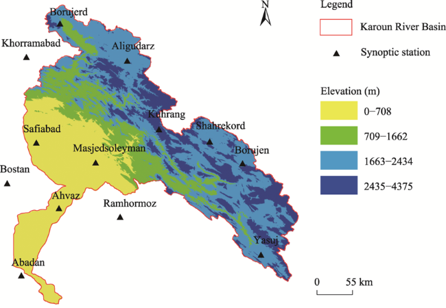
Fig. 1 Location and spatial distribution of synoptic stations in the Karoun River Basin (KRB)
Table 1 Brief description of 13 synoptic stations in the Karoun River Basin (KRB)
Synoptic station Elevation (m) Average annual precipitation (mm) Annual average temperature (°C) Climate type
Abadan 6.6 174.3 25.9 Extra-arid
Ahvaz 22.5 238.0 26.0 Arid
Aligudarz 2022.1 394.8 13.2 Mediterranean
Borujen 2260.0 255.2 12.8 Semi-arid
Borujerd 1629.0 473.5 14.9 Mediterranean
Bostan 7.8 211.3 24.1 Arid
Khorramabad 1147.8 487.9 16.7 Semi-arid
Kuhrang 2365.0 1406.8 9.9 Humid
Masjedsoleyman 320.5 457.2 25.0 Semi-arid
Ramhormoz 150.5 330.1 27.5 Arid
Safiabad 82.9 349.5 24.6 Semi-arid
Shahrekord 2048.9 327.3 11.9 Semi-arid
Yasuj 1816.3 886.0 15.0 Humid

Note: Classification of climate type is based on Rahimi et al. (2013).

2.2 NASA Earth Exchange Global Daily Downscaled Projections (NEX-GDDP) dataset

The NEX-GDDP dataset consists of downscaled climatic data, including precipitation, maximum temperature, and minimum temperature, at a spatial resolution of 0.25°×0.25° and a daily scale. These data were derived from the CMIP5 GCMs. The historical data span from 1950 to 2005 and the future data are during 2009-2099 under RCP4.5 and RCP8.5 scenarios. In the NEX-GDDP dataset, we correcting and downscaling data have been done using the Bias-Correction Spatial Disaggregation (BCSD) method based on the Global Meteorological Forcing Dataset (GMFD) as observational climate data (Wood et al., 2002, 2004; Sheffield et al., 2006). This study provides a basic description of implementing the BCSD method to downscale the CMIP5 GCM data in the NEX-GDDP dataset. Fuller exposition of the BCSD method can be found in Thrasher et al. (2012) and Thrasher and Nemani (2015). The BCSD method consists of three main steps: preprocessing, bias-correction, and spatial disaggregation. In the bias-correction step, the bias of GCM data is corrected by comparing GCM data with GMFD historical data and finding a transfer function. The cumulative distribution function (CDF) of GMFD data and the CDF of retrospective GCM simulations are generated, and then the two cumulative distribution functions are compared. GCM values in any CDF quantile can be translated to corresponding GMFD values in the same CDF quantile. The main assumption in correcting climate data in the future is that the CDF of the GCM simulations is stable across the retrospective and prospective periods. The spatial disaggregation interpolates the bias-corrected future GCM data from the GMFD data (0.25°×0.25°). The processes of spatial disaggregation include subtracting the coarse-scale spatial patterns of GMFD data from the bias-corrected future data to get the bias-corrected temporal scaling factors for each grid in the future period, interpolating temporal scaling factors from coarse-scale to targeted resolution (0.25°×0.25°), and adding the temporal scaling factors at the targeted resolution to the fine-scale spatial patterns of GMFD data (Thrasher et al., 2012). A total of seven GCMs from the NEX-GDDP dataset were used in this study, and their characteristics are described in Table 2. Data downloaded from the Google Earth Engine (GEE) web platform (https://earthengine.google.com/) can process various data sets including the NEX-GDDP under RCP4.5 and RCP8.5 scenarios during the periods of 2009-2039, 2040-2069, and 2070-2099.
Table 2 Details and characteristics of Global Climate Models (GCMs) used in this study
NEX-GDDP
resolution
Original
resolution
Center GCM
0.25°×0.25° 2.80°×2.80° Canadian Centre for Climate Modelling and Analysis in Canada CanESM2
0.25°×0.25° 0.94°×1.25° National Center for Atmospheric Research in the United States CCSM4
0.25°×0.25° 1.40°×1.40° National Centre for Meteorological Research in France CNRM-CM5
0.25°×0.25° 2.00°×2.50° National Oceanic and Atmospheric Administration (NOAA),
geophysical fluid dynamics laboratory in the United States
GFDL-CM3
0.25°×0.25° 1.25°×2.50° Institute Pierre-Simon Laplace in France IPSL-CM5A-MR
0.25°×0.25° 1.40°×1.40° Meteorological Research Institute in Japan MRI-CGCM3
0.25°×0.25° 1.40°×1.40° Atmosphere and Ocean Research Institute in the University of Tokyo, National Institute for Environmental Studies, and Japan Agency for Marine-Earth Science and Technology in Japan MIROC5

Note: GCM, Global Climate Model; CanESM2, Canadian Earth System Model version 2; CCSM4, Community Climate System Model version 4; CNRM-CM5, Center National for Research Meteorological Climate Model version 5; GFDL-CM3, Geophysical Fluid Dynamics Laboratory Coupled Model version 3; IPSL-CM5A-MR, Institute Pierre Simon Laplace Climate Model phase 5 Atmospheric Mid Resolution; MRI-CGCM3, Meteorological Research Institute Coupled Global Climate Model version 3; MIROC5, Model for Interdisciplinary Research on Climate version 5; NEX-GDDP, NASA Earth Exchange Global Daily Downscaled Projections.

2.3 Evaluation indices

In this study, statistical metrics including correlation coefficient (CC; Pearson, 1896), root mean square error (RMSE; Hyndman and Koehler, 2006), standard deviation (SD; Pearson, 1894), and coefficient of variation (CV; Brown, 1998) were used to evaluate the performance of GCMs in estimating SPI. These evaluation indices can be calculated using the following equations:
$\text{CC}=\frac{\sum\limits_{i=1}^{N}{({{O}_{i}}-\bar{O})({{G}_{i}}-\bar{G})}}{\sqrt{\sum\limits_{i=1}^{N}{{{({{O}_{i}}-\bar{O})}^{2}}\sum\limits_{i=1}^{N}{{{({{G}_{i}}-\bar{G})}^{2}}}}}}$,
$\text{RMSE}=\sqrt{\frac{1}{N}\sum\limits_{i=1}^{N}{\mathop{(\mathop{O}_{i}-\mathop{G}_{i})}^{2}}}$,
$\text{SD}=\sqrt{\frac{\sum\limits_{i=1}^{N}{{{({{G}_{i}}-\bar{G})}^{2}}}}{N-1}}$,
$\text{CV}=\frac{\text{SD}}{{\bar{G}}}$,
where N is the sample size; Oi is SPI calculated from synoptic stations datasets in month i; Gi is SPI calculated from GCMs in month i; and $\bar{O}$ and $\bar{G}$ represent the mean values of synoptic stations datasets and GCMs, respectively.

2.4 Uncertainty analysis

We used Bootstrap algorithm to investigate the formation of uncertainty bounds. Bootstrap algorithm is a non-parametric, powerful, and computer-based resampling method for statistical inference without relying on too many assumptions. Bootstrap algorithm has the same idea as the Monte Carlo method, but one of its advantages is that it does not make any assumptions concerning the distribution of data used (Padiyedath Gopalan et al., 2019; Wilks, 2019). In this method, uncertainty bounds are calculated by sampling the original data, repeating this process in large numbers (usually 1000 times), and calculating the mean and variance for each iteration. The workflow of Bootstrap algorithm is as follows: firstly, drawing a sample from the original data with replacement; secondly, calculating and storing the mean (or any other statistic metrics) of the resampled values; thirdly, repeating the previous two steps n times (n is a large number such as 1000); fourthly, computing the mean of the calculated sample statistics; lastly, constructing a sampling distribution with these Bootstrap statistics and using it to make further statistical inferences such as obtaining uncertainty bounds. For more details, refer to Efron (1979), Efron and Gong (1983), and Efron and Tibshirani (1993).

2.5 Classification of Standard Precipitation Index (SPI)

SPI was developed by McKee et al. (1993) to assign a numerical value to precipitation for characterizing meteorological drought and comparing regions with different climates. Low computational complexity and flexibility over timescales are two prominent features of this index (Sternberg et al., 2011). Also, SPI is effective for analyzing wet periods and cycles as well as dry periods and cycles as it is normalized (Wu et al., 2001; SPI, 2020; Chikabvumbwa et al., 2022). SPI only needs precipitation values to describe drought and reflect the effect of drought on water resources, groundwater reserves, soil moisture, and river regime (Edwards, 1997). The calculation of SPI relies on fitting the gamma probability density function to the precipitation dataset (McKee et al., 1993). In this study, the software from National Drought Mitigation Center has been used to calculate SPI, which is freely available at https://drought.unl.edu/Monitoring/SPI/SPIPro gram.aspx. This study considers the one-month timescale for SPI calculation. Furthermore, we categorized SPI values according to the study conducted by McKee et al. (1993) (Table 3).
Table 3 Classification of dry and wet conditions based on Standard Precipitation Index (SPI)
Classification SPI Classification SPI
Near normal -0.50≤SPI≤0.00 Near normal 0.00≤SPI≤0.50
Abnormally dry -0.70≤SPI< -0.50 Abnormally wet 0.50<SPI≤0.70
Moderately dry -1.20≤SPI< -0.70 Moderately wet 0.70<SPI≤1.20
Severely dry -1.50≤SPI< -1.20 Severely wet 1.20<SPI≤1.50
Extremely dry -2.00≤SPI< -1.50 Extremely wet 1.50<SPI≤2.00
Exceptionally dry SPI< -2.00 Exceptionally wet SPI>2.00

Note: Classification of SPI is based on McKee et al. (1993).

3 Results and discussion

3.1 Performance of Global Climate Models (GCMs) for estimating SPI during historical period

In this study, seven bias-corrected GCMs from the NEX-GDDP datasets were considered for drought analysis. We evaluated the reliability of the historical GCMs in estimating SPI based on statistical metrics. The spatial distribution of RMSE and CC of SPI calculated based on GCMs and synoptic station as well as the spatial distribution of SD of SPI calculated from each GCM are shown in Figure 2. Findings indicate that the best performance in estimating SPI is assigned to the Meteorological Research Institute Coupled Global Climate Model version 3 (MRI-CGCM3). Because the RMSE value is less than 0.75 in 77% of the synoptic stations. In addition, the SPI estimated by MRI-CGCM3 is in good agreement with the SPI calculated based on synoptic stations, and the value of CC is more than 0.60 in all stations. As presented in Figure 2, models with lower performance include Center National for Research Meteorological Climate Model version 5 (CNRM-CM5), Community Climate System Model version 4 (CCSM4), and Institute Pierre Simon Laplace Climate Model phase 5 Atmospheric Mid Resolution (IPSL-CM5A-MR). The average value of RMSE in these models is high and more than 0.66. In contrast, the range of RMSE in MRI-CGCM3 is between 0.53 and 0.71, with an average value of 0.58. Other GCMs, including Canadian Earth System Model version 2 (CanESM2), Geophysical Fluid Dynamics Laboratory Coupled Model version 3 (GFDL-CM3), and Model for Interdisciplinary Research on Climate version 5 (MIROC5), have an appropriate performance. In these models (CanESM2, GFDL-CM3, and MIROC5), the value of CC obtained between the observed time series of SPI and the GCM time series of SPI is more than 0.61 in 70% of the synoptic stations, and the RMSE value is less than 0.65 in 50% of the synoptic stations. It should be noted that all models except IPSL-CM5A-MR are suitable in Southwest KRB. The value of SD in synoptic stations located in Southwest KRB is between 0.55 and 0.75. In contrast, the value of SD is higher in north and northeast synoptic stations, indicating that SPI in these areas is more dispersed. In addition, the average value of CC in this area is always more than 0.62, and RMSE is less than 0.59.
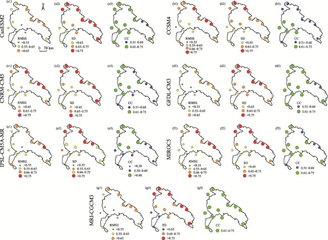
Fig. 2 Spatial distribution of root mean square error (RMSE) and correlation coefficient (CC) of SPI calculated based on Global Climate Models (GCMs) and synoptic stations as well as spatial distribution of standard deviation (SD) of SPI calculated from each Global Climate Model (GCM). (a1-a3), Canadian Earth System Model version 2 (CanESM2); (b1-b3), Community Climate System Model version 4 (CCSM4); (c1-c3), Center National for Research Meteorological Climate Model version 5 (CNRM-CM5); (d1-d3), Geophysical Fluid Dynamics Laboratory Coupled Model version 3 (GFDL-CM3); (e1-e3), Institute Pierre Simon Laplace Climate Model phase 5 Atmospheric Mid Resolution (IPSL-CM5A-MR); (f1-f3), Model for Interdisciplinary Research on Climate version 5 (MIROC5); (g1-g3), Meteorological Research Institute Coupled Global Climate Model version 3 (MRI-CGCM3).
Due to the wide disparity among models, climate change projections are highly uncertain, leading to a significant impact on experts and managers who obtain climate change information. In this study, we used seven GCMs to reduce model uncertainty and increase their efficiency. The spatial distribution of CC, RMSE, and SD of SPI calculated from the average of all GCMs and observations is shown in Figure 3. Results indicate that the average of all GCMs leads to a significantly increasing correlation between calculated SPI and observed SPI. In more than 76% of the synoptic stations, the value of CC between both datasets (average of all GCMs and observations) is always higher than 0.75; and in other stations, it ranges from 0.66 to 0.75. Findings based on RMSE illustrate that the errors in estimating SPI tend to decline when the average of all GCMs is used. For example, the lowest average value of RMSE among different models over the KRB is equal to 0.61, while using the average of all GCMs, the average value of RMSE decreases by about 21% (equal to 0.48). In addition, the calculation error of SPI in the highlands of the basin has been reduced, with the value of RMSE decreasing by about 18% to 0.43. Furthermore, considering several GCMs instead of one GCM, the uncertainty has been decreased so that the range of SD reaches 0.46-0.65.
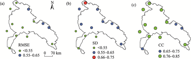
Fig. 3 Spatial distribution of RMSE (a), SD (b), and CC (c) of SPI calculated from the average of all GCMs and observations

3.2 Uncertainty analysis of GCMs in estimating SPI

In order to evaluate the uncertainty, we calculated CV of all GCMs (Fig. 4). Results show that CCSM4 and MIROC5 have lower uncertainty. The CV of CCSM4 and MIROC5 is 3.50 in 85% and 54% of the synoptic stations, respectively. However, Song et al. (2020) showed that MIROC5 has the highest uncertainty in estimating precipitation compared with the other GCMs. Therefore, although MIROC5 has high uncertainty in estimating precipitation, its uncertainty in drought analysis may be small. In contrast, based on CV value, CanESM2, IPSL-CM5A-MR, and MRI-CGCM3 have higher uncertainty in more than 50% of the synoptic stations. Therefore, it is recommended to use these models to estimate SPI and monitor drought.
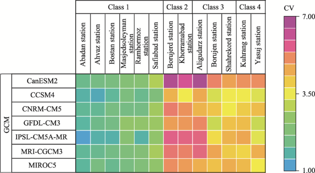
Fig. 4 Matrix plot of coefficient of variation (CV) between GCMs and synoptic stations. Class 1 (-4.0-700.0 m), Class 2 (700.0-1660.0 m), Class 3 (1660.0-2430.0 m), and Class 4 (2430.0-4375.0 m) are four distinct elevation classes that are divided based on the Shuttle Radar Topography Mission (SRTM) Digital Elevation Model (DEM).
It can be seen from Figure 4 that the uncertainty is unevenly distributed in space. As shown in Figure 4, the uncertainty of all GCMs tends to increase in the north, east, and southeast of the basin, including Aligudarz, Borujen, Borujerd, Khorramabad, Kuhrang, Shahrekord, and Yasuj stations; while in other regions, the uncertainty is lower. The results demonstrate that the performance of GCMs in estimating SPI is slightly improved and the uncertainty of the model is reduced by reducing the elevation to the range of Class 1. In addition, this trend is more obvious in CanESM2 and IPSL-CM5A-MR (Fig. 4). Among different models, CCSM4 and MIROC5 have a better performance and are positively correlated with the observed data in most elevation classes, and the values of CV and CC are always less than 4.50 and higher than 0.51, respectively.
In addition, we calculated uncertainty bounds of each GCM using the non-parametric Bootstrap algorithm. The results of 95% uncertainty bounds of each GCM for each station are presented in Table 4. It can be seen that CCSM4 has fewer uncertainty bounds in 69% of the synoptic stations. For example, the uncertainty bounds of CCSM4 in Ahvaz, Safiabad, and Shahrekord stations are 0.36-0.52, 0.21-0.39, and 0.10-0.31, respectively; while the uncertainty bounds of CanESM2 in Ahvaz, Safiabad, and Shahrekord stations are 0.23-0.41, 0.14-0.34, and 0.06-0.28, respectively (Table 4). The results show that different GCMs have various responses in estimating SPI and meteorological drought analysis. Similarly, Wu et al. (2021) found that the most significant uncertainty contribution in drought projections comes from GCMs. Bias-correction method can also reduce this uncertainty, especially in the northern hemisphere. The results demonstrate that the width of uncertainty bounds is very high in elevated areas.
Table 4 Results of 95% uncertainty bounds of each GCM for 13 synoptic stations during historical period
Synoptic station GCM
Borujerd Borujen Aligudarz Ahvaz Abadan
0.00-0.24 0.04-0.26 -0.01-0.23 0.23-0.41 0.24-0.42 CanESM2
0.07-0.29 0.12-0.32 0.06-0.28 0.36-0.52 0.31-0.48 CCSM4
0.04-0.26 0.08-0.29 0.07-0.29 0.26-0.44 0.27-0.44 CNRM-CM5
0.06-0.28 0.12-0.33 0.04-0.27 0.24-0.42 0.30-0.47 GFDL-CM3
0.02-0.25 0.09-0.30 0.03-0.25 0.32-0.48 0.48-0.62 IPSL-CM5A-MR
0.03-0.26 0.06-0.28 0.03-0.25 0.25-0.43 0.27-0.45 MRI-CGCM3
0.05-0.27 0.08-0.29 0.07-0.28 0.22-0.40 0.28-0.45 MIROC5
Ramhormoz Masjedsoleyman Kuhrang Khorramabad Bostan GCM
0.19-0.38 0.20-0.38 0.05-0.27 0.01-0.25 0.21-0.40 CanESM2
0.25-0.43 0.21-0.40 0.10-0.31 0.10-0.31 0.28-0.45 CCSM4
0.22-0.41 0.22-0.41 0.08-0.30 0.05-0.27 0.22-0.40 CNRM-CM5
0.18-0.37 0.17-0.37 0.07-0.29 0.05-0.28 0.23-0.41 GFDL-CM3
0.31-0.48 0.19-0.38 0.06-0.28 0.02-0.25 0.32-0.48 IPSL-CM5A-MR
0.20-0.39 0.21-0.39 0.09-0.30 0.04-0.26 0.23-0.41 MRI-CGCM3
0.20-0.39 0.22-0.40 0.07-0.29 0.05-0.27 0.25-0.43 MIROC5
Yasuj Shahrekord Safiabad GCM
0.05-0.27 0.06-0.28 0.14-0.34 CanESM2
0.11-0.32 0.10-0.31 0.21-0.39 CCSM4
0.07-0.29 0.10-0.31 0.16-0.35 CNRM-CM5
0.13-0.33 0.08-0.29 0.16-0.36 GFDL-CM3
0.11-0.32 0.07-0.28 0.18-0.37 IPSL-CM5A-MR
0.07-0.28 0.08-0.29 0.15-0.35 MRI-CGCM3
0.10-0.31 0.06-0.28 0.18-0.37 MIROC5
Time series of SPI along with their uncertainty bounds among GCMs is presented in Figure 5. Due to the large outputs, only the time series of the average of GCMs and observations in each elevation class, namely Class 1 (Ramhormoz station), Class 2 (Khorramabad station), Class 3 (Borujen station), and Class 4 (Kuhrang station), is shown. As shown in Figure 5, GCMs tend to underestimate SPI variability, especially when capturing extreme dry and wet events (Fig. 5c). The temporal variability of SPI tends to be smaller in the Ramhormoz station (Fig. 5a). The results demonstrate that predictions are far less reliable when only one or a limited number of GCMs are considered to assess climate change. These results are in good agreement with some studies comparing multiple GCMs, which have highlighted the significant reliance on models for prediction (Sunyer et al., 2015; Osuch et al., 2016; Xu et al., 2019; Wu et al., 2020). Sunyer et al. (2015) assessed and compared six GCMs. They concluded the large variability in climate models and recommended using a set of climate models for prediction. Overall, it is clear that using the average of GCMs has acceptable efficiency in capturing wet and dry events in wet and dry years. Therefore, the results of validation process show that the NEX-GDDP can be considered as a valuable dataset for the analysis of meteorological drought and the simulation of wet and dry conditions.
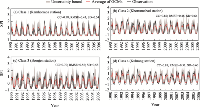
Fig. 5 Time series of SPI in each elevation class during 1990-2005. (a), Class 1 (Ramhormoz station); (b), Class 2 (Khorramabad station); (c), Class 3 (Borujen station); (d), Class 4 (Kuhrang station).

3.3 Projection of drought conditions based on SPI

In order to further understand the possible drought and wetness occurred in the KRB, we also analyzed the drought and wetness frequency for each station under RCP4.5 and RCP8.5 scenarios during historical and future periods (Figs. 6 and 7). According to Figure 6, the areas most affected by drought are the northern regions. However, the wetness frequency is higher than drought frequency over the basin during the historical period, especially in the upper and middle basin. Accordingly, the range of wetness frequency in these regions is between 41% and 45% (Fig. 7). In contrast, the magnitude of drought frequency varies from 5% to 35%. Under RCP4.5 and RCP8.5 scenarios, drought frequency shows an increasing pattern in North KRB. Drought frequency during 2070-2099 is slightly more than that during 2009-2039 and 2040-2069. Compared with RCP4.5, the increase of drought frequency under RCP8.5 scenario covers a wider range of the basin.
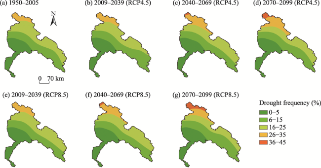
Fig. 6 Spatial distribution of drought frequency during 1990-2005 (a), 2009-2039 (b and e), 2040-2069 (c and f), and 2070-2099 (d and g) under RCP4.5 and RCP8.5 scenarios
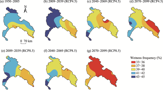
Fig. 7 Spatial distribution of wetness frequency during 1990-2005 (a), 2009-2039 (b and e), 2040-2069 (c and f), and 2070-2099 (d and g) under RCP4.5 and RCP8.5 scenarios
Unlike drought frequency, it is quite evident that the magnitude of wetness frequency decreases with time. It should be noted that although there is an increasing trend under RCP4.5 scenario during 2009-2039, wetness frequency decreases significantly during other periods. Results demonstrate that lower wetness frequency varies from 37% to 39% and covers about 25% of the KRB area during historical period. The area with the lowest wetness frequency is equivalent 31% and 19% of the basin area under RCP4.5 and RCP8.5 scenarios during 2040-2069, respectively. During 2070-2099, under RCP4.5 and RCP8.5 scenarios, the area with wetness frequencies of 35% to 37% increases to 19% and 77%, respectively. Therefore, central, northern, and eastern regions of the basin are likely to have a lower wetness frequency during this period. According to the study conducted by Soltani et al. (2016), which examined the changes in precipitation across Iran during 1975-2010, they found that the largest downward trend was seen in the western part of the country. As the reduction of precipitation is one of the reasons for the intensification of drought in the region, it can be said that this phenomenon is consistent with the results of this study.
Overall, the projected change in drought and wetness frequency has shown an increase in drought and a decline in wetness events, which can eventually reduce water stock and resources of the basin. Therefore, if decision-makers do not take effective measures to reduce drought and its consequences, the north, east, and southeast parts of the KRB will face significant damage from agricultural, social, economic, and other sectors. In addition, given that flood and drought are two extremes of a hydrological cycle (Ward et al., 2020), in several regions of the USA and Australia, drought has led to devastating floods and severely affected the environment and economy (Van Dijk et al., 2013; Vahedifard et al., 2017). It is important to consider the interactions between these closely-linked phenomena in the forthcoming study in order to manage and reduce damages in this basin.
We calculated the average of SPI during historical and future periods under RCP4.5 and RCP8.5 scenarios in each climatological season, including spring, summer, autumn, and winter. The results of six synoptic stations are shown in Figure 8.
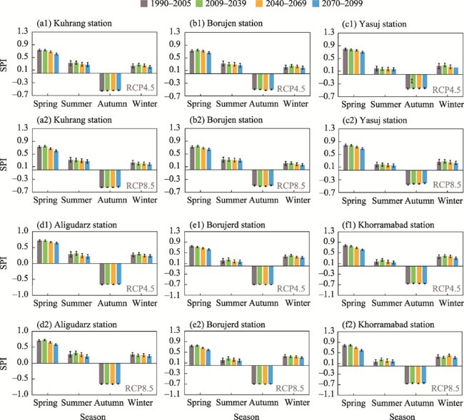
Fig. 8 Seasonal variations of SPI under RCP4.5 and RCP8.5 scenarios in Kuhrang (a1 and a2), Borujen (b1 and b2), Yasuj (c1 and c2), Aligudarz (d1 and d2), Borujerd (e1 and e2), and Khorramabad (f1 and f2) stations. Bars represent standard errors.
The results show that the GCMs projections have significant seasonal changes. The value of SPI in Kuhrang station during historical period under RCP4.5 scenario is equal to 0.73, while the value decreases by 0.5%, 7.8%, and 16.5% during 2009-2039, 2040-2069, and 2070-2099, respectively, under RCP4.5 scenario. The value of SPI increases by 2.0%, 8.5%, and 17.6% under RCP8.5 scenario during 2009-2039, 2040-2069, and 2070-2099, respectively. It should be noted that the decreasing trend is more conspicuous in northern regions (including Aligudarz, Borujerd, and Khorramabad stations). As indicated by Haile et al. (2019, 2020), drought trends have increased in spring, which is consistent with the results of this study. In summer, the value of SPI has generally decreased with time, but its intensity is lower than that in spring. As shown in Figure 8, autumn is most affected by dry events, and the average value of SPI for all periods in this season is negative. The important point is that the change of drought index in autumn does not follow a specific trend, and in many stations, the change is not significant. These results are consistent with the study conducted by Ababaei and Ramezani Etedali (2019), who investigated the spatiotemporal variations of drought indices in Iran. Their results show that there is no significant trend in the value of SPI in autumn in western and southwestern Iran. Based on the results, although SPI increased from 2009 to 2039, it shows a downward trend in winter during 2040-2069 and 2070-2099 compared with the historical period. The average value of SPI in Yasuj station is estimated to be about 0.26 in winter during historical period. During 2009-2039, 2040-2069, and 2070-2099, SPI is 0.29, 0.27, and 0.21 under RCP4.5 scenario, respectively; and it is 0.28, 0.25, and 0.23 under RCP8.5 scenario, respectively. The decrease of SPI in winter may mean that the number or intensity of dry periods in this season increases. The projected trend is of highly relevant to agriculture and water management and may severely affect these sectors. The decrease of SPI in winter is due to insufficient precipitation, which will lead to a reduction in the recharge of underground aquifer. Therefore, owing to the changes of agricultural water resources and the reduced availability of soil moisture, rainfed agriculture is affected and the production and crop yields are reduced, thus increasing crop damage. As a result, the economy and livelihood of the majority of the rural inhabitants and farmers who heavily rely on rainfed subsistence agriculture will be seriously damaged. Therefore, the impact on the future agricultural is likely to be mostly negative under RCP4.5 and RCP8.5 scenarios. The higher average SPI value is seen in spring, so it is recommended to plant in spring to reduce agricultural damages of climate change in the KRB. To sum up, it can be said that drought monitoring under climate change scenarios on a seasonal scale is more necessary and applicable than that on an annual scale. On the other hand, the changes in drought and wetness events may be due to global warming, and are likely attributed to decreased precipitation or increased temperature (Dai, 2013). Therefore, it is suggested to consider the role of other parameters in the future research.

4 Conclusions

Climate change makes it cumbersome to understand the future meteorological drought characteristics on the regional scale. In addition, investigating the drought patterns under climate change scenarios is vital to address various risks of future drought. In this study, we used SPI to conduct a special study on the meteorological drought conditions under RCP4.5 and RCP8.5 scenarios in southwestern Iran at one-month timescale. The results illustrate that MRI-CGCM3 depicts the best results and has the highest CC and the lowest RMSE in all synoptic stations compared with the observed SPI during historical period. In contrast, the least performance belongs to CNRM-CM5, CCSM4, and IPSL-CM5A. According to the results, the performance of GCMs is unevenly in space, and GCMs used in this study have varios uncertainty degrees in different elevation classes for drought index estimation. As a result, using the average of a few GCMs to minimize uncertainties and errors is recommended. Uncertainty analysis of the impacts of climate change on drought shows that the projected drought under RCP8.5 has more uncertainties during 2009-2039 and 2040-2069. Based on the results, some regions like the northern parts of KRB will suffer from an increase in drought frequency, and regions such as the east and center parts of the basin will experience a decrease in the frequency of wet events in the future. The results of this study can be used to develop adaptation and mitigation plans to deal with the risks caused by climate change in Southwest Iran. Since the results of this study may change due to various occurrences of natural climate variability, these findings should be considered as possible events affected by future climate.

Acknowledgements

The authors are thankful to the NASA Ames Research Center for preparing the NEX-GDDP dataset. The authors also give appreciation to the reviewers for their thoughtful comments and suggestions, which helped to improve this manuscript.
[1]
Ababaei B, Ramezani Etedali H. 2019. Investigating climate change over 1957-2016 in an arid environment with three drought indexes. Theoretical and Applied Climatology, 137: 2977-2992.

[2]
Adamson P, Bird J. 2010. The Mekong: A drought-prone tropical environment? International Journal of Water Resources Development, 26(4): 579-594.

[3]
Aziz A, Umar M, Mansha M, et al. 2018. Assessment of drought conditions using HJ-1A/1B data: a case study of Potohar region, Pakistan. Geomatics, Natural Hazards and Risk, 9(1): 1019-1036.

[4]
Bhalme H N, Mooley D A. 1980. Large-scale droughts/floods and monsoon circulation. Monthly Weather Review, 108(8): 1197-1211.

[5]
Bower E, Meneghetti L, O'Connor K. 2015. Global Estimates 2015: People Displaced by Disasters. [2022-04-24]. https://www.internal-displacement.org/publications/global-estimates-2015-people-displaced-by-disasters.

[6]
Brown C E. 1998. Coefficient of variation. In: Brown C E. Applied Multivariate Statistics in Geohydrology and Related Sciences. Heidelberg: Springer.

[7]
Cao F Q, Gao T. 2019. Effect of climate change on the centennial drought over China using high-resolution NASA-NEX downscaled climate ensemble data. Theoretical and Applied Climatology, 138(1-2): 1189-1202.

[8]
Chikabvumbwa S R, Salehnia N, Manzanas R, et al. 2022. Assessing the effect of spatial-temporal droughts on dominant crop yield changes in Central Malawi. Environmental Monitoring and Assessment, 194: 63, doi: 10.1007/s10661-021-09709-4.

[9]
Cook B I, Ault T R, Smerdon J E. 2015. Unprecedented 21st century drought risk in the American Southwest and Central plains. Science Advances, 1(1), doi: 10.1126/sciadv.1400082.

[10]
Dai A. 2013. Increasing drought under global warming in observations and models. Nature Climate Change, 3(1): 52-58.

[11]
Das S, Das J, Umamahesh N V. 2021. Identification of future meteorological drought hotspots over Indian region: A study based on NEX-GDDP data. International Journal of Climatology, 41(12): 5644-5662.

[12]
Dehghan S, Salehnia N, Sayari N, et al. 2020. Prediction of meteorological drought in arid and semi-arid regions using PDSI and SDSM: A case study in Fars Province, Iran. Journal of Arid Land, 12(2): 318-330.

[13]
Edwards D C. 1997. Characteristics of 20th Century Drought in the United States at Multiple Time Scales. Colorado: Colorado State University.

[14]
Efron B. 1979. Bootstrap methods: another look at the Jackknife. The Annals of Statistics, 7(1): 1-26.

[15]
Efron B, Gong G. 1983. A leisurely look at the bootstrap, the Jackknife, and cross-validation. The American Statistician, 37(1): 36-48.

[16]
Efron B, Tibshirani R J. 1993. An Introduction to the Bootstrap. New York: Chapman and Hall Press.

[17]
Fattahi E, Habibi M, Kouhi M. 2015. Climate change impact on drought intensity and duration in West of Iran. Journal of Earth Science & Climatic Change, 6(10), doi: 10.4172/2157-7617.1000319.

[18]
Feng S, Trnka M, Hayes M, et al. 2017. Why do different drought indices show distinct future drought risk outcomes in the U.S. great plains? Journal of Climate, 30(1): 265-278.

[19]
Fooladi M, Golmohammadi M H, Safavi H R, et al. 2021. Fusion-based framework for meteorological drought modeling using remotely sensed datasets under climate change scenarios: Resilience, vulnerability, and frequency analysis. Journal of Environmental Management, 297: 113283, doi: 10.1016/j.jenvman.2021.113283.

[20]
Gaitán E, Monjo R, Pórtoles J, et al. 2020. Impact of climate change on drought in Aragon (NE Spain). Science of the Total Environment, 740: 140094, doi: 10.1016/j.scitotenv.2020.140094.

[21]
Gibbs W J, Maher J V. 1967. Rainfall Deciles as Drought Indicates. Melbourne: Bureau of Meteorology Press.

[22]
Haile G G, Tang Q, Sun S, et al. 2019. Droughts in East Africa: causes, impacts and resilience. Earth-Science Reviews, 193: 146-161.

[23]
Haile G G, Tang Q, Hosseini Moghari S M, et al. 2020. Projected impacts of climate change on drought patterns over East Africa. Earth's Future, 8(7), doi: 10.1029/2020EF001502.

[24]
Hayes M, Svoboda M, Wall N, et al. 2011. The lincoln declaration on drought indices: universal meteorological drought index recommended. Bulletin of the American Meteorological Society, 92(4): 485-488.

[25]
Hyndman R J, Koehler A B. 2006. Another look at measures of forecast accuracy. International Journal of Forecasting, 22(4): 679-688.

[26]
Ionita M, Scholz P, Chelcea S. 2016. Assessment of droughts in Romania using the standardized precipitation index. Natural Hazards, 81: 1483-1498.

[27]
IPCC Intergovernmental Panel on Climate Change. 2013. Climate change 2013:the physical science basis. In:Contribution of Working Group I to the Fifth Assessment Report of the Intergovernmental Panel on Climate Change. Geneva, Switzerland.

[28]
Karamouz M, Nazif S, Falahi M. 2013. Hydrology and Hydroclimatology Principles and Applications (1st ed.). Florida: CRC Press.

[29]
Khan J U, Islam A K M S, Das M K, et al. 2020. Future changes in meteorological drought characteristics over Bangladesh projected by the CMIP 5 multi-model ensemble. Climatic Change, 162(2): 667-685.

[30]
Li Y S, Lu H, Yang K, et al. 2021. Meteorological and hydrological droughts in Mekong river basin and surrounding areas under climate change. Journal of Hydrology: Regional Studies, 36: 100873, doi: 10.1016/j.ejrh.2021.100873.

[31]
Madani K. 2014. Water management in Iran: what is causing the looming crisis? Journal of Environmental Studies and Sciences, 4(4): 315-328.

[32]
Maraun D. 2016. Bias correcting climate change simulations - a critical review. Current Climate Change Reports, 2: 211-220.

[33]
McKee T B, Doesken N J, Kleist J. 1993. The relationship of drought frequency and duration to time scales. In:8th Conference on Applied Climatology. Anaheim, USA.

[34]
Mirgol B, Nazari M, Ramezani Etedali H, et al. 2021. Past and future drought trends, duration, and frequency in the semi-arid Urmia lake basin under a changing climate. Meteorological Applications, 28(4): 1-19.

[35]
Modarresi Rad A, AghaKouchak A, Navari M, et al. 2021. Progress, challenges, and opportunities in remote sensing of drought. In: Wu H, Lettenmaier D P, Tang Q H, et al. Global Drought and Flood: Observation, Modeling, and Prediction. Global Drought and Flood: Observation, Modeling, and Prediction. Massachusetts: American Geophysical Union.

[36]
Nam W H, Hayes M J, Svoboda M D, et al. 2015. Drought hazard assessment in the context of climate change for South Korea. Agricultural Water Management, 160: 106-117.

[37]
Noorisameleh Z, Khaledi S, Shakiba A, et al. 2020. Comparative evaluation of impacts of climate change and droughts on river flow vulnerability in Iran. Water Science and Engineering, 13(4): 265-274.

[38]
Osuch M, Romanowicz R J, Lawrence D, et al. 2016. Trends in projections of standardized precipitation indices in a future climate in Poland. Hydrology and Earth System Sciences, 20(5): 1947-1969.

[39]
Padiyedath Gopalan S, Kawamura A, Amaguchi H, et al. 2019. A bootstrap approach for the parameter uncertainty of an urban-specific rainfall-runoff model. Journal of Hydrology, 579, doi: 10.1016/j.jhydrol.2019.124195.

[40]
Pearson K. 1894. On the dissection of asymmetrical frequency curves. Philosophical Transactions of the Royal Society A, 185: 71-100.

[41]
Pearson K. 1896. Mathematical contributions to the theory of evolution-on a form of spurious correlation which may arise when indices are used in the measurement of organs. Proceedings of the Royal Society of London, 60: 489-498.

[42]
Rahimi J, Ebrahimpour M, Khalili A. 2013. Spatial changes of extended De Martonne climatic zones affected by climate change in Iran. Theoretical and Applied Climatology, 112: 409-418.

[43]
Salehnia N, Hosseini F, Farid A, et al. 2019. Comparing the performance of dynamical and statistical downscaling on historical run precipitation data over a semi-arid region. Asia-Pacific Journal of Atmospheric Sciences, 55: 737-749.

[44]
Salehnia N, Salehnia N, Saradari Torshizi A, et al. 2020. Rainfed wheat (Triticum aestivum L.) yield prediction using economical, meteorological, and drought indicators through pooled panel data and statistical downscaling. Ecological Indicators, 111, doi: 10.1016/j.ecolind.2019.105991.

[45]
Schwalm C R, Anderegg W R L, Michalak A M, et al. 2017. Global patterns of drought recovery. Nature, 548: 202-205.

[46]
Sheffield J, Goteti G, Wood E F. 2006. Development of a 50-year high-resolution global dataset of meteorological forcings for land surface modeling. Journal of Climate, 19: 3088-3111.

[47]
Shelton M. 2018. Hydroclimatology Perspectives and Applications. Cambridge: Cambridge University Press.

[48]
Soltani M, Laux P, Kunstmann H, et al. 2016. Assessment of climate variations in temperature and precipitation extreme events over Iran. Theoretical and Applied Climatology, 126(3-4): 775-795.

[49]
Song Y H, Chung E S, Shiru M S. 2020. Uncertainty analysis of monthly precipitation in GCMs using multiple bias correction methods under different RCPs. Sustainability, 12(18), doi: 10.3390/su12187508.

[50]
SPI Standardized Precipitation Index. 2020. Copernicus European Drought Observatory Report, European Commission, Joint Research Centre. [2022-01-10]. https://edo.jrc.ec.europa.eu/documents/factsheets/factsheet_spi.pdf.

[51]
Sternberg T, Thomas D, Middleton N. 2011. Drought dynamics on the Mongolian steppe, 1970-2006. International Journal of Climatology, 31(12): 1823-1830.

[52]
Sunyer M A, Hundecha Y, Lawrence D, et al. 2015. Inter-comparison of statistical downscaling methods for projection of extreme precipitation in Europe. Hydrology and Earth System Sciences, 19(4): 1827-1847.

[53]
Thrasher B, Maurer E P, McKellar C, et al. 2012. Technical Note: Bias correcting climate model simulated daily temperature extremes with quantile mapping. Hydrology and Earth System Sciences, 16(9): 3309-3314.

[54]
Thrasher B, Nemani R. 2015. NASA Earth Exchange Global Daily Downscaled Projections (NEX-GDDP) Dataset. [2022-01-25]. https://www.nasa.gov/nex/gddp.

[55]
Vaghefi S A, Keykhai M, Jahanbakhshi F, et al. 2019. The future of extreme climate in Iran. Scientific Reports, 9(1), doi: 10.1038/s41598-018-38071-8.

[56]
Vahedifard F, AghaKouchak A, Ragno E, et al. 2017. Lessons from the Oroville dam. Science, 355(6330): 1139-1140.

[57]
Vaittinada Ayar P, Vrac M, Bastin S, et al. 2016. Intercomparison of statistical and dynamical downscaling models under the EURO- and MED-CORDEX initiative framework: present climate evaluations. Climate Dynamics, 46: 1301-1329.

[58]
Van Dijk A I J M, Beck H E, Crosbie R S, et al. 2013. The millennium drought in southeast Australia (2001-2009): natural and human causes and implications for water resources, ecosystems, economy, and society. Water Resources Research, 49(2): 1040-1057.

[59]
Vicente-Serrano S M, Beguería S, López-Moreno J I. 2010. A multiscalar drought index sensitive to global warming: the standardized precipitation evapotranspiration index. Journal of Climate, 23(7): 1696-1718.

[60]
Wang J S, Wang W, Cheng H, et al. 2021. Propagation from meteorological to hydrological drought and its influencing factors in the Huaihe River Basin. Water, 13(14), doi: 10.3390/w13141985.

[61]
Ward P J, Marleen C D R, Mård J, et al. 2020. The need to integrate flood and drought disaster risk reduction strategies. Water Security, 11, doi: 10.1016/j.wasec.2020.100070.

[62]
WMO World Meteorological Organization, GWP (Global Water Partnership). 2016. Handbook of Drought Indicators and Indices. [2022-01-25]. https://library.wmo.int/doc_num.php?explnum_id=3057.

[63]
Wilby R L, Harris I. 2006. A framework for assessing uncertainties in climate change impacts: low flow scenarios for the river Thames, UK. Water Resources Research, 420(2), doi: 10.1029/2005WR004065.

[64]
Wilhite D A. 2000. Drought as a Natural Hazard:Concepts and Definitions. Drought:A Global Assessment. Nebraska: Nebraska University Press.

[65]
Wilks D S. 2019. Statistical Methods in the Atmospheric Sciences. [2022-01-25]. https://www.sciencedirect.com/book/9780128158234/statistical-methods-in-the-atmospheric-sciences.

[66]
Wood A W, Maurer E P, Kumar A, et al. 2002. Long-range experimental hydrologic forecasting for the eastern United States. Journal of Geophysical Research-Atmospheres, 107, doi: 10.1029/2001JD000659.

[67]
Wood A W, Leung L R, Sridhar V, et al. 2004. Hydrologic implications of dynamical and statistical approaches to downscaling climate model outputs. Climatic Change, 62: 189-216.

[68]
Wu C, Yeh P J F, Chen Y Y, et al. 2020. Future precipitation-driven meteorological drought changes in the CMIP 5 multi-model ensembles under 1.5°C and 2°C global warming. Journal of Hydrometeorology, 21(9): 2177-2196.

[69]
Wu C, Yeh P J F, Ju J, et al. 2021. Assessing the spatiotemporal uncertainties in future meteorological droughts from CMIP 5 models, emission scenarios, and bias corrections. Journal of Climate, 34(5): 1903-1922.

[70]
Wu H, Hayes M J, Weiss A, et al. 2001. An evaluation of the standardized precipitation index, the China-Z index and the statistical Z-score. International Journal of Climatology, 21(6): 745-758.

[71]
Xu B B, Ju J L, Wu C H, et al. 2019. Projection and uncertainty of precipitation extremes in the CMIP5 multimodel ensembles over nine major basins in China. Atmospheric Research, 226: 122-137.

Outlines

/