• SUN Huaizhang ,
  • ZHAO Xueqiang ,
  • CHEN Yangbo , * ,
  • LIU Jun
展开

收稿日期: 2024-07-15

  修回日期: 2024-12-21

  录用日期: 2024-12-25

  网络出版日期: 2025-08-13

Impacts of extreme climate and vegetation phenology on net primary productivity across the Qinghai- Xizang Plateau, China from 1982 to 2020

  • SUN Huaizhang ,
  • ZHAO Xueqiang ,
  • CHEN Yangbo , * ,
  • LIU Jun
Expand
  • School of Geography and Planning, Sun Yat-sen University, Guangzhou 510275, China
*CHEN Yangbo (E-mail: )

Received date: 2024-07-15

  Revised date: 2024-12-21

  Accepted date: 2024-12-25

  Online published: 2025-08-13

本文引用格式

SUN Huaizhang , ZHAO Xueqiang , CHEN Yangbo , LIU Jun . [J]. Journal of Arid Land, 2025 , 17(3) : 350 -367 . DOI: 10.1007/s40333-025-0075-x

Abstract

The net primary productivity (NPP) is an important indicator for assessing the carbon sequestration capacities of different ecosystems and plays a crucial role in the global biosphere carbon cycle. However, in the context of the increasing frequency, intensity, and duration of global extreme climate events, the impacts of extreme climate and vegetation phenology on NPP are still unclear, especially on the Qinghai-Xizang Plateau (QXP), China. In this study, we used a new data fusion method based on the MOD13A2 normalized difference vegetation index (NDVI) and the Global Inventory Modeling and Mapping Studies (GIMMS) NDVI3g datasets to obtain a NDVI dataset (1982-2020) on the QXP. Then, we developed a NPP dataset across the QXP using the Carnegie-Ames-Stanford Approach (CASA) model and validated its applicability based on gauged NPP data. Subsequently, we calculated 18 extreme climate indices based on the CN05.1 dataset, and extracted the length of vegetation growing season using the threshold method and double logistic model based on the annual NDVI time series. Finally, we explored the spatiotemporal patterns of NPP on the QXP and the impact mechanisms of extreme climate and the length of vegetation growing season on NPP. The results indicated that the estimated NPP exhibited good applicability. Specifically, the correlation coefficient, relative bias, mean error, and root mean square error between the estimated NPP and gauged NPP were 0.76, 0.17, 52.89 g C/(m2•a), and 217.52 g C/(m2•a), respectively. The NPP of alpine meadow, alpine steppe, forest, and main ecosystem on the QXP mainly exhibited an increasing trend during 1982-2020, with rates of 0.35, 0.38, 1.40, and 0.48 g C/(m2•a), respectively. Spatially, the NPP gradually decreased from southeast to northwest across the QXP. Extreme climate had greater impact on NPP than the length of vegetation growing season on the QXP. Specifically, the increase in extremely-wet-day precipitation (R99p), simple daily intensity index (SDII), and hottest day (TXx) increased the NPP in different ecosystems across the QXP, while the increases in the cold spell duration index (CSDI) and warm spell duration index (WSDI) decreased the NPP in these ecosystems. The results of this study provide a scientific basis for relevant departments to formulate future policies addressing the impact of extreme climate on vegetation in different ecosystems on the QXP.

1 Introduction

The net primary productivity (NPP) refers to the amount of new carbon fixed through photosynthesis by a plant community per unit of time and space (Liu et al., 2019b). It is not only a crucial indicator of vegetation dynamics and the net carbon exchange between the atmosphere and terrestrial ecosystems, but also plays an important role in the global biosphere carbon cycle (Liu et al., 2019b; Cuo et al., 2021). According to the report of the Intergovernmental Panel on Climate Change (IPCC), the frequency, intensity, and duration of global extreme climate events will increase rapidly in the 21st century, and their impact range will further expand (Ye et al., 2020). Extreme climate events are likely to cause more severe, prolonged, and irreversible damage to terrestrial ecosystems due to the limited adaptability of terrestrial ecosystems (Ciais et al., 2005). In addition, as a result of climate warming, the length of vegetation growing season in the Northern Hemisphere has been extended, which could allow more time for plants to photosynthesis, thereby increasing the amount of carbon they fix from the atmosphere (Piao et al., 2007; Dragoni et al., 2011). Therefore, it is vital to fully and accurately understand and assess the impacts of extreme climate and the length of vegetation growing season on NPP.
Traditional methods for estimating the NPP primarily rely on field measurements, which can provide relatively accurate NPP data at small scales (Clark et al., 2001; Wei et al., 2022). However, they are difficult to be widely applied in large spatial scale and long time series studies due to limitations in manpower, time, and cost (Xu et al., 2020). With the development of remote sensing technology, estimating the NPP based on remote sensing data and mathematical models has become an important method for obtaining large spatial scale, long time series, and high temporal resolution NPP datasets, and this method has been widely used in Romania (Prăvălie et al., 2023), Shaanxi Province, China (Wei et al., 2022), and the Yangtze River Basin, China (Yang et al., 2021). In recent years, most studies have primarily focused on the spatiotemporal patterns and influencing factors of NPP (Zhu et al., 2020; Ge et al., 2021). Research on the temporal trends of NPP has mainly been conducted at the pixel-by-pixel scales of nations, provinces, cities, or even small regions (Yang et al., 2021; Wei et al., 2022). In addition, studies on the spatial analysis of NPP have primarily explored the distribution of high and low NPP values and the regions with increasing or decreasing NPP trends (Xue et al., 2023; Yin et al., 2024). A recent comprehensive study showed that the average annual NPP of marshes on the Qinghai-Xizang Plateau (QXP) increased significantly by 11.70 (±1.07) g C/(m2•10a) from 2000 to 2020 (Shen et al., 2022b). In addition, some studies have found that from 2000 to 2018, the average NPP of the permafrost and non-permafrost regions on the QXP increased at rates of 1.52 and 1.22 g C/(m2•a), respectively (Li et al., 2022). Current research on the factors influencing the NPP has mainly focused on the relationship of NPP with precipitation and temperature (Chen et al., 2014; Wei et al., 2022). Precipitation and temperature can directly and indirectly affect the NPP by influencing the community biomass and plant metabolism (Michaletz et al., 2014). Chen et al. (2014) reported that climate change and anthropogenic activities were the main driving forces of the increase in the actual NPP of grasslands on the QXP during the periods 1982-2001 and 2002-2011, respectively.
Different types of extreme climate events on the QXP had varying impacts on vegetation growth (Wang et al., 2018; Liu et al., 2019a). Specifically, extreme wet events can promote vegetation growth, while drought, extreme high temperatures, and extreme low temperatures significantly inhibit vegetation growth in different regions. Previous studies have indicated that up to 80% of extreme vegetation growth decline events across the QXP have been associated with extreme climate events related to moisture and temperature (Piao et al., 2024). Currently, several studies have been conducted on the spatiotemporal distribution and driving factors of NPP across the QXP (Chen et al., 2014; Li et al., 2022), but few studies have explored the correlations of NPP with extreme climate and the length of the growing season. As the highest and most extensive plateau in the world, the QXP is considered to be a premonitory region for global climate change (Ye et al., 2020). The ecosystems on the QXP are highly sensitive to climate change and can be easily damaged by extreme climate events. According to historical environmental experience, vegetation must implement balanced strategies to achieve optimal growth under the current environmental conditions (Li et al., 2021a). However, such strategies are not optimal under extreme climatic conditions (Li et al., 2021a). Although vegetation typically stores sufficient non-structural carbohydrates to recover from occasional damage, repeated damage can weaken the competitive ability of some species (Li et al., 2021a). Previous studies have indicated that extreme climate events may affect the structure, composition, and functioning of terrestrial ecosystems, thereby affecting the carbon cycle and its feedback to the climate system (Frank et al., 2015). In addition, under the influence of global climate change, the length of vegetation growing season is increasing, which may lead to an increase in the NPP (Sun et al., 2019; Ye et al., 2020). Hence, it is necessary to explore the correlations of NPP with extreme climate and the length of vegetation growing season across the QXP, which is of great significance for further understanding the impacts of extreme climate and the length of vegetation growing season on NPP in this region.
In this study, we developed a NPP dataset for the QXP from 1982 to 2020 using the Carnegie-Ames-Stanford Approach (CASA) model, calculated 18 extreme climate indices based on the CN05.1 dataset, and extracted the length of vegetation growing season using the threshold method and double logistic model according to the annual normalized difference vegetation index (NDVI) time series. Our primary aims were to investigate the spatiotemporal patterns of NPP on the QXP from 1982 to 2020 and analyze the impacts of extreme climate and the length of vegetation growing season on NPP.

2 Materials and methods

2.1 Study area

The QXP (Fig. 1), which is located in Southwest China, covers an area of approximately 2.57×10⁶ km2 and has an average elevation of more than 4000 m a.s.l. (Sun et al., 2022). Because of the abundant glaciers, snow, and fresh water, it is often referred to as the Third Pole and the Water Tower of Asia (Ji et al., 2015). Generally, with the impacts of monsoonal winds from the Indian Ocean and elevation, the climate on the QXP is characterized by thermal and moisture gradients from southeast to northwest (Chen et al., 2015). Specifically, due to its distinctive topographic and landscape features, the winter weather on the QXP is dominated by the westerly jet, which brings dry air and high winds. In summer, precipitation and temperature increase as a result of the profound effects of the South Asian and East Asian monsoons (Yong et al., 2021). In recent decades, numerous studies have reported significant increasing or decreasing trends of a series of extreme warm/cold temperature indices on the QXP (Zhang et al., 2011b; Yin et al., 2019). Furthermore, existing research has shown that the start of vegetation growing season on the QXP advanced by 9.4 (±2.2) and 8.3 (±2.0) d during the periods 1982-1999 and 2000-2020, respectively (Shen et al., 2022a).
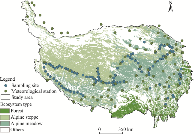
Fig. 1 Overview of the Qinghai-Xizang Plateau (QXP) and distributions of meteorological stations and sampling sites. Ecosystem type data are based on the vegetation type data sourced from the Resource and Environmental Science Data Platform (https://www.resdc.cn/data.aspx?DATAID=122).

2.2 Data sources

Regarding the data used in this study, the monthly sunshine duration (h) for the period 1982-2020 from 93 national standard meteorological stations were obtained from the Chinese Meteorological Administration (http://data.cma.cn/). The daily maximum temperature (°C), daily minimum temperature (°C), daily mean temperature (°C), and daily precipitation (mm) data were obtained from the CN05.1 dataset (https://ccrc.iap.ac.cn/resource/detail?id=228), with a spatial resolution of 0.25°. The NDVI datasets used in this study included the Moderate Resolution Imaging Spectroradiometer (MODIS) NDVI dataset (2001-2020) and the Global Inventory Modeling and Mapping Studies (GIMMS) NDVI3g dataset (1982-2015) derived from the Advanced Very High Resolution Radiometer (AVHRR). Specifically, we produced the MODIS NDVI dataset (MOD13A2 NDVI in this study) at a 1-km resolution and 16-d compositing period based on a sophisticated algorithm and quality control (https://ladsweb.modaps.eosdis.nasa.gov/). The GIMMS NDVI3g dataset has a spatial resolution of 0.083° and a temporal resolution of 2 weeks (https://data.tpdc.ac.cn/en/). In addition, the aboveground biomass data were derived from 115 sampling sites across the QXP in 2015 (Fig. 1).

2.3 Methods

The workflow of this study is shown in Figure 2. First, we developed a NPP dataset for the QXP from 1982 to 2020 using the CASA model based on monthly precipitation, monthly temperature, monthly NDVI, monthly sunshine duration, and vegetation type data, and evaluated the applicability of the estimated NPP dataset based on gauged NPP data. Next, we calculated 12 extreme temperature indices and 6 extreme precipitation indices based on daily precipitation, daily minimum temperature, and daily maximum temperature data from the CN05.1 dataset, and extracted the length of vegetation growing season using the threshold method and double logistic model based on the annual NDVI time series. Then, we investigated the spatiotemporal patterns of NPP across the QXP using the Sen's trend estimation and Mann-Kendall significance test. Last, we explored the impact mechanisms of extreme climate and the length of vegetation growing season on NPP using the random forest (RF) model and SHapley Additive exPlanations (SHAP) method. Data statistics and mapping analyses were carried out according to different ecosystem types of the forest, alpine meadow, alpine steppe, and main ecosystem (including forest, alpine meadow, and alpine steppe).
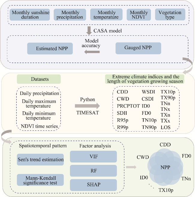
Fig. 2 Flowchart of this study. NDVI, normalized difference vegetation index; CASA, Carnegie-Ames-Stanford Approach; NPP, net primary productivity; CDD, consecutive dry days; CWD, consecutive wet days; PRCPTOT, total wet-day precipitation; SDII, simple daily intensity index; R95p, very-wet-day precipitation; R99p, extremely-wet-day precipitation; WSDI, warm spell duration index; CSDI, cold spell duration index; ID0, ice days; FD0, frost days; TN10p, cool nights; TN90p, warm nights; TX10p, cool days; TX90p, warm days; TNn, coldest night; TNx, warmest night; TXn, coldest day; TXx, hottest day; LOS, length of vegetation growing season; VIF, Variance Inflation Factor; RF, random forest; SHAP, SHapley Additive exPlanations.

2.3.1 Calculation of extreme climate indices

Based on the daily precipitation, daily maximum temperature, and daily minimum temperature datasets, we calculated 6 extreme precipitation indices (consecutive dry days (CDD), consecutive wet days (CWD), total wet-day precipitation (PRCPTOT), simple daily intensity index (SDII), very-wet-day precipitation (R95p), and extremely-wet-day precipitation (R99p)) and 12 extreme temperature indices (warm spell duration index (WSDI), cold spell duration index (CSDI), ice days (ID0), frost days (FD0), cool nights (TN10p), warm nights (TN90p), cool days (TX10p), warm days (TX90p), coldest night (TNn), warmest night (TNx), coldest day (TXn), and hottest day (TXx)) to reflect the intensity, frequency, and duration of extreme climate events across the QXP. The definitions and abbreviations of extreme climate indices are shown in Tables 1 and 2.
Table 1 Definitions of extreme precipitation indices
Index Unit Description
Consecutive dry days (CDD) d Maximum number of consecutive days with daily precipitation <1 mm
Consecutive wet days (CWD) d Maximum number of consecutive days with daily precipitation ≥1 mm
Total wet-day precipitation (PRCPTOT) mm Annual total precipitation on wet days
Simple daily intensity index (SDII) mm/d Annual total precipitation divided by the number of wet days in the year
Very-wet-day precipitation (R95p) mm Annual total precipitation of days with daily precipitation >95th percentile
Extremely-wet-day precipitation (R99p) mm Annual total precipitation of days with daily precipitation >99th percentile

Note: 95th percentile and 99th percentile represent 95th percentile and 99th percentile of precipitation on wet days for the period 1982-2020, respectively. Precise definitions are given at https://etccdi.pacificclimate.org/list_27_indices.shtml.

Table 2 Definitions of extreme temperature indices
Index Unit Description
Warm spell duration index (WSDI) d Number of days with at least six consecutive days when TX>90th percentile
Cold spell duration index (CSDI) d Number of days with at least six consecutive days when TN<10th percentile
Ice days (ID0) d Number of days when TX<0°C
Frost days (FD0) d Number of days when TN<0°C
Cool nights (TN10p) % Percentage of days when TN<10th percentile
Warm nights (TN90p) % Percentage of days when TN>90th percentile
Cool days (TX10p) % Percentage of days when TX<10th percentile
Warm days (TX90p) % Percentage of days when TX>90th percentile
Coldest night (TNn) °C Minimum of TN
Warmest night (TNx) °C Maximum of TN
Coldest day (TXn) °C Minimum of TX
Hottest day (TXx) °C Maximum of TX

Note: TX and TN denote the daily maximum temperature and daily minimum temperature, respectively. The 10th percentile denotes the calendar day 10th percentile centred on a 5-d window for the base period 1982-2020. The 90th percentile denotes the calendar day 90th percentile centred on a 5-d window for the base period 1982-2020. Precise definitions are given at https://etccdi.pacificclimate.org/ list_27_indices.shtml.

2.3.2 Time extension method for GIMMS NDVI3g

The main vegetation index products currently used for estimating the NPP include the MODIS NDVI and GIMMS NDVI3g (Ye et al., 2020; Yang et al., 2021). Although the two NDVI datasets are recognized as effective indices for monitoring vegetation dynamics at different spatial scales, their applications are often constrained by their respective periods. Due to the differing qualities of these two NDVI datasets, they often cannot be used together directly. Hence, in this study, we developed a new fusion method based on the MODIS NDVI and GIMMS NDVI3g datasets to obtain a long-term NDVI dataset. Blending the MODIS NDVI and GIMMS NDVI3g datasets has become a popular method for extending the period of the GIMMS NDVI3g dataset (Zhang et al., 2011a). A widely used method for achieving this is upscaling the MODIS NDVI dataset using average filtering and then calibrating the upscaled data through time-series regression to match the GIMMS NDVI3g dataset. This method has been proven to be effective, but it has the notable problem of oversimplifying the spatial response during the upscaling. Specifically, average filtering-based upscaling assumes that the coarse-resolution pixel is only related to the fine-resolution pixels that are spatially covered by it, which is incorrect. The actual spatial response is much more complicated because some fine pixels beyond the coverage of a coarse pixel still influence it in scale-transform tasks. Therefore, in this study, we developed a new method for fusing MOD13A2 NDVI and GIMMS NDVI3g data and extended the period of the GIMMS NDVI3g dataset to 2020. This method can be expressed using the formula as follows:
$G=a\left(P_{n} \times M^{p}\right)+b,$
where G is the simulated NDVI based on MOD13A2 NDVI and GIMMS NDVI3g datasets (GIMMS-MOD13A2 NDVI); a and b are the linear calibration coefficients; Pn is the normalized two-dimensional Gaussian kernel; M is the MOD13A2 NDVI; and Mp is the patch of M, referred to as the receptive field of G.

2.3.3 NPP estimation using the CASA model

In this study, the CASA model was used to estimate the NPP across the QXP (Ye et al., 2020; Hou et al., 2023). The CASA model is a light use efficiency model based on multiple datasets (i.e., monthly precipitation, monthly temperature, vegetation type, monthly NDVI, and monthly sunshine duration), and it has been widely used to estimate the NPP at different regional scales (Yan et al., 2018; He et al., 2022; Li et al., 2023). The formulas are as follows:
$\operatorname{NPP}(x, t)=\operatorname{APAR}(x, t) \times \varepsilon(x, t),$
$\operatorname{APAR}(x, t)=\operatorname{SOL}(x, t) \times \operatorname{FPAR}(x, t) \times 0.5,$
$\operatorname{FPAR}_{\mathrm{NDVI}}(x, t)=\frac{\left(\operatorname{NDVI}(x, t)-\mathrm{NDVI}_{(i, \min )}\right) \times\left(\mathrm{FPAR}_{\max }-\mathrm{FPAR}_{\min }\right)}{\operatorname{NDVI}_{(i, \max )}-\operatorname{NDVI}_{(i, \min )}}+\operatorname{FPAR}_{\text {min }},$
$\operatorname{FPAR}_{\mathrm{SR}}(x, t)=\frac{\left(\mathrm{SR}(x, t)-\mathrm{SR}_{(i, \min )}\right) \times\left(\mathrm{FPAR}_{\text {max }}-\mathrm{FPAR}_{\text {min }}\right)}{\mathrm{SR}_{(i, \max )}-\mathrm{SR}_{(i, \min )}}+\mathrm{FPAR}_{\text {min }},$
$\operatorname{SR}(x, t)=\frac{1+\operatorname{NDVI}(x, t)}{1-\operatorname{NDVI}(x, t)},$
$\operatorname{FPAR}(x, t)=\left(\operatorname{FPAR}_{\mathrm{NDVI}}(x, t)+\operatorname{FPAR}_{\mathrm{SR}}(x, t)\right) \times 0.5,$
$\varepsilon(x, t)=T_{\varepsilon 1}(x, t) \times T_{\varepsilon 2}(x, t) \times W_{\varepsilon}(x, t) \times \varepsilon_{\max },$
$T_{\varepsilon 1}(x, t)=0.8+0.02 \times T_{\mathrm{opt}}(x)-0.0005\left[T_{\mathrm{opt}}(x)\right]^{2},$
$\begin{aligned}T_{\varepsilon 2}(x, t)= & 1.1814 /\left\{1+\exp \left[0.2 \times\left(T_{\text {opt }}(x)-10-T(x, t)\right)\right]\right\}, \\& /\left\{1+\exp \left[0.3 \times\left(-T_{\text {opt }}(x)-10+T(x, t)\right)\right]\right\}\end{aligned}$
$W_{\varepsilon}(x, t)=0.5+0.5 \times E(x, t) / E_{p}(x, t),$
where NPP(x,t) is the estimated NPP (g C/m2); APAR is the photosynthetic active radiation absorbed by green vegetation (MJ/m2); ε is the actual light use efficiency (g C/MJ); SOL is the solar radiation (MJ/m2); FPAR is the absorption ratio of the vegetation layer to the incident photosynthetic active radiation; NDVI(i,min) and NDVI(i,max) are the minimum and maximum NDVI of the ith vegetation type, respectively; FPARmax and FPARmin are 0.950 and 0.001, respectively; SR(i,min) and SR(i,max) are the minimum and maximum values of Simple Ratio vegetation index of the ith vegetation type, respectively; Tε1 and Tε2 are the stresses of low and high temperatures on the light use efficiency, respectively; Wε is the water stress coefficient; εmax is the maximum light use efficiency under ideal conditions (g C/MJ); Topt is the air temperature in the month when the NDVI reaches the maximum for the year (°C); T is the air temperature (°C); E is the estimated evapotranspiration (mm); and Ep is the potential evapotranspiration (mm).
The detailed calculation process of the CASA model has been discussed in a previous study (Gao et al., 2012). To ensure the reliability of the estimated NPP, in this study, we compared the estimated NPP using the CASA model with actual gauged NPP data. Here, the gauged NPP was obtained via conversion of the aboveground biomass in 2015. The specific steps are as follows: (1) we calculated the belowground biomass based on the ratio of the belowground to aboveground biomass for alpine meadow (7.92), alpine steppe (4.25), and alpine desert steppe (7.89); and (2) the sum of the belowground and aboveground biomass was taken as the total biomass, which was multiplied by a coefficient of 0.45 to obtain gauged NPP with carbon unit (Ye et al., 2020).

2.3.4 Determination of the length of vegetation growing season

In this study, the TIMESAT software was used to extract phenological metrics across the QXP during 1982-2020. The TIMESAT program was developed for analyzing time series of satellite sensor data and extracting phenological and seasonal parameters (Jönsson and Eklundh, 2002). It provides three different smoothing functions for fitting time series data, namely, double logistic, Savitzky-Golay, and asymmetric Gaussian functions (Jönsson and Eklundh, 2004). In this study, the double logistic model was adopted to fit the annual NDVI time series data after many trials and comparisons. Then, the threshold method in the TIMESAT was used to extract the vegetation phenology. The start and end thresholds of vegetation growing season were set to 0.2 and 0.5, respectively.

2.3.5 Sen's trend estimation

Sen's trend estimation is a mathematical statistical method used to quantitatively describe the trends of time series data (Sen, 1968). The formula is as follows:
$\beta=\operatorname{median}\left(\frac{X_{l}-X_{k}}{l-k}\right), l>k,$
where β is the Sen's slope of the time series; and Xl and Xk are the two data points in the series corresponding to the lth and kth year, respectively. β>0 indicates an increasing trend and β<0 indicates a decreasing trend. Because Sen's trend estimation lacks statistical significance testing, we used the Mann-Kendall significance test method to evaluate the significance of the trends. The detailed calculation method for the Mann-Kendall significance test was discussed in a previous study (Hou et al., 2023).

2.3.6 Construction of RF model

The RF model was proposed by Breiman (2001) and has been widely applied to classification and regression problems due to its excellent performance. This model can overcome multicollinearity and overfitting issues, especially for high-dimensional data (Chen et al., 2021), thus having been widely used in ecology and hydrology (Li et al., 2021b; Wang et al., 2021). The RF model generally uses the bootstrap sampling method to extract multiple samples from the original dataset (Wang et al., 2021; Li et al., 2024). Each bootstrap sample is used to create a decision tree, and then, these decision trees are combined to obtain the final result through a voting score rule (Breiman, 2001; Liu et al., 2024). In this study, the dataset was split into 70% for training and 30% for validation in the RF model.

2.3.7 Factor importance analysis based on the SHAP method

The RF model often achieves a better predictive accuracy than traditional statistical models, but it loses the interpretability that statistical models offer. Therefore, the SHAP method was used in this study based on the RF model. The SHAP was originally proposed by Lundberg and Lee (2017) and designed for describing the performance of a machine learning model based on game theory and local explanations (Wang et al., 2021). It assigns specific predictive importance values to each feature, ensuring robust global and local interpretability. For a specific input sample z with M features, the Shapley additive mechanism expresses an individual prediction by decomposing it into feature contributions as follows (Wang et al., 2022):
$f(z)=g\left(z^{\prime}\right)=\varphi_{0}+\sum_{j=1}^{M} \varphi_{j} z_{j}^{\prime},$
where f and g are the original model and explanation model, respectively, and g should match the output of the original model for a simplified input $z^{\prime}$ of z; $\varphi_{0}$ is the mean value of the prediction values; and $\varphi_{j} z_{j}^{\prime}$ is the SHAP value for feature j in sample z. In this study, the mean absolute SHAP values were calculated to describe the importance of extreme climate indices and the length of the growing season to NPP. Higher values indicate a greater impact on NPP.

3 Results

3.1 Accuracy assessment of the simulated GIMMS-MOD13A2 NDVI and estimated NPP

To validate the effectiveness of the new data fusion method proposed in this paper, we conducted a comparative analysis of the simulated GIMMS-MOD13A2 NDVI and GIMMS NDVI3g for 2001, 2005, 2010, and 2015. The linear regression results revealed that there was a high degree of similarity between the simulated GIMMS-MOD13A2 NDVI and GIMMS NDVI3g for 2001, 2005, 2010, and 2015, with R2 values of 0.89, 0.89, 0.88, and 0.90, respectively (Fig. 3). Moreover, the slopes of the fitted lines for 2001, 2005, 2010, and 2015 were 0.989, 0.978, 0.974, and 0.987, respectively. Overall, the simulated GIMMS-MOD13A2 NDVI dataset exhibited a certain level of reliability.
Fig. 3 Linear relationship between the GIMMS-MOD13A2 NDVI and GIMMS NDVI3g in 2001 (a), 2005 (b), 2010 (c), and 2015 (d). GIMMS, Global Inventory Modeling and Mapping Studies. GIMMS-MOD13A2 NDVI is the simulated NDVI based on MOD13A2 NDVI and GIMMS NDVI3g datasets.
By comparing the estimated NPP using the CASA model with the actual gauged NPP data in 2015, we found that the estimated NPP dataset had strong reliability across the QXP (Fig. 4). Specifically, the correlation coefficient, relative bias, mean error, and root mean square error between the estimated NPP and gauged NPP were 0.76, 0.17, 52.89, and 217.52 g C/(m2•a), respectively.
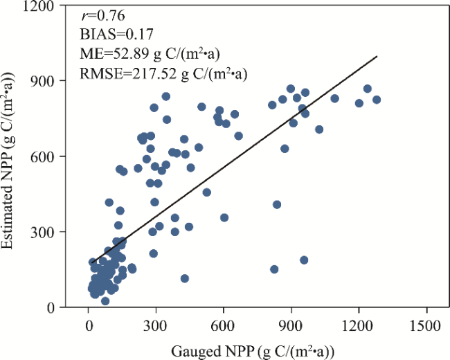
Fig. 4 Linear relationship between the gauged and estimated NPP data. r, BIAS, ME, and RMSE denote the correlation coefficient, relative bias, mean error, and root mean square error, respectively.

3.2 Spatiotemporal patterns of NPP across the QXP

At the regional scale, the NPP in different ecosystems on the QXP generally increased during the period 1982-2020 (Fig. 5). Specifically, the NPP of the alpine meadow exhibited a non-significant increasing trend with a rate of 0.35 g C/(m2•a). Conversely, the NPP of the alpine steppe, forest, and main ecosystem increased significantly at rates of 0.38, 1.40, and 0.48 g C/(m2•a), respectively.
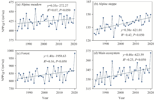
Fig. 5 Temporal variations in NPP in different ecosystems on the QXP from 1982 to 2020. (a), alpine meadow; (b), alpine steppe; (c), forest; (d), main ecosystem.
The spatial pattern and temporal trends of NPP on the QXP exhibited pronounced spatial heterogeneity from 1982 to 2020 (Fig. 6). The multi-year average NPP decreased from southeast to northwest. The lowest value occurred in the northwest, and the highest value occurred in the southeast (Fig. 6a). In addition, the multi-year average NPP was highest in the forest, followed by the alpine meadow, main ecosystem, and alpine steppe (Fig. 6b). Moreover, in most areas on the QXP, the NPP exhibited an increasing trend during 1982-2020. The higher rates of increase were primarily concentrated in the southeast (Fig. 6c). Furthermore, the mean Sen's slope of NPP was highest in the forest, followed by the main ecosystem, alpine steppe, and alpine meadow (Fig. 6d).
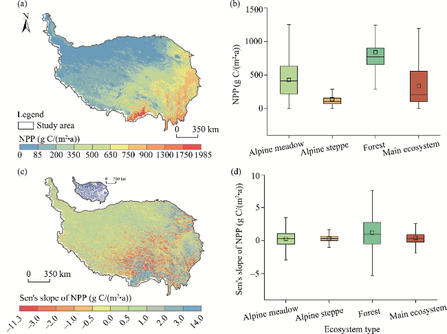
Fig. 6 Spatial patterns and zonal statistics of multi-year average NPP (a and b) and Sen's slope of NPP (c and d) on the QXP during 1982-2020. The inset in the upper left corner of Figure 6c shows that the colored pixels experienced significant changes (P<0.050 level). In the box plots, the box boundaries denote the 25th and 75th percentiles, the line in the box denotes the median, the square in the box denotes the average value, and whiskers below and above the box denote the Q1-1.5(Q3-Q1) and Q3+1.5(Q3-Q1).

3.3 Spatiotemporal patterns of the length of vegetation growing season across the QXP

The multi-year average length of vegetation growing season decreased from southeast to northwest. The lowest value occurred in the northwest, and the highest value was found in the southeast (Fig. 7a). In addition, the multi-year average length of vegetation growing season was highest in the forest, followed by the alpine meadow, main ecosystem, and alpine steppe (Fig. 7b). Moreover, from 1982 to 2020, in most areas of the QXP, the length of vegetation growing season exhibited an increasing trend, and the higher rates of increase were primarily concentrated in the eastern region of the QXP (Fig. 7c). Furthermore, the mean Sen's slope of the length of vegetation growing season was highest in the forest, followed by the alpine meadow, main ecosystem, and alpine steppe (Fig. 7d).
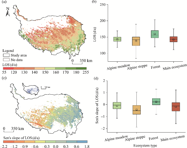
Fig. 7 Spatial patterns and zonal statistics of the multi-year average LOS (a and b) and Sen's slope of LOS (c and d) on the QXP during 1982-2020. The inset in the upper left corner of Figure 7c shows that the colored pixels experienced significant changes (P<0.050 level). In the box plots, the box boundaries denote the 25th and 75th percentiles, the line in the box denotes the median, the square in the box denotes the average value, and whiskers below and above the box denote the Q1-1.5(Q3-Q1) and Q3+1.5(Q3-Q1).

3.4 Impacts of extreme climate and the length of vegetation growing season on NPP across the QXP

Figure 8 shows the mean absolute SHAP values of extreme climate indices and the length of vegetation growing season. The top six factors influencing the NPP of the alpine meadow were R99p, TXx, SDII, CSDI, WSDI, and TXn, with mean absolute SHAP values of 0.039, 0.035, 0.027, 0.025, 0.017, and 0.012, respectively. In addition, the R99p was the factor with the greatest impact on NPP in the alpine steppe, with a mean absolute SHAP value of 0.042, followed by the SDII (0.025), CSDI (0.016), TXx (0.013), WSDI (0.012), and TXn (0.010). For the forest, the mean absolute SHAP values of the TXx, WSDI, CSDI, SDII, TN90p, and CDD were 0.032, 0.024, 0.017, 0.016, 0.014, and 0.011, respectively. In addition, the R99p had the greatest impact on NPP in the main ecosystem, with a mean absolute SHAP value of 0.053, followed by the SDII (0.032), CSDI (0.028), TXx (0.026), CDD (0.018), and WSDI (0.017).
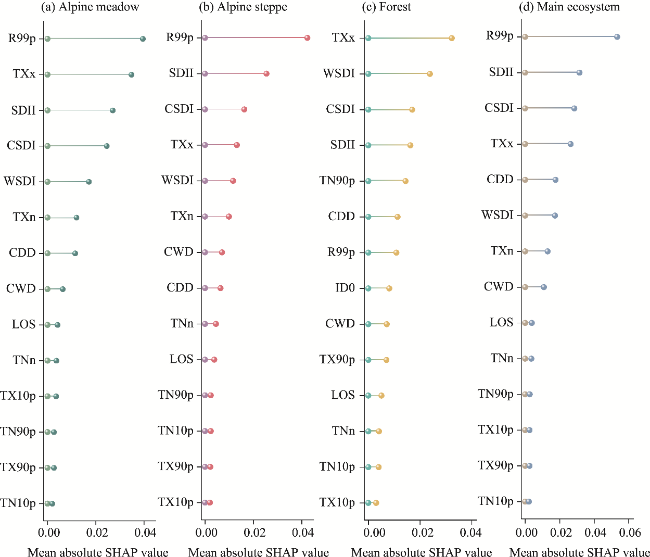
Fig. 8 Relative importances of extreme climate indices and the length of vegetation growing season based on the mean absolute SHAP values
In the alpine meadow, the NPP increased with R99p (R2=0.51, P<0.001), TXx (R2=0.42, P<0.001), and SDII (R2=0.49, P<0.001) within a certain range (Fig. 9). However, the NPP exhibited significant negative correlations with CSDI (R2=0.39, P<0.001) and WSDI (R2=0.15, P<0.001) in the alpine meadow. In the alpine steppe, the NPP increased with R99p (R2=0.51, P<0.001), SDII (R2=0.47, P<0.001), and TXx (R2=0.18, P<0.001). In contrast, the NPP exhibited significant negative correlations with CSDI (R2=0.12, P<0.001) and WSDI (R2=0.27, P<0.001). In the forest, the results indicated that the NPP was positively correlated with TXx (R2=0.19, P<0.001) and SDII (R2=0.19, P<0.001) within a certain range, while it exhibited significant negative correlations with WSDI (R2=0.11, P<0.001), CSDI (R2=0.07, P<0.001), and TN90p (R2=0.10, P<0.001). In addition, the relationship between the NPP and R99p in the main ecosystem was similar to that between the NPP and R99p in the alpine meadow. The NPP in the main ecosystem exhibited significant positive correlations with SDII (R2=0.59, P<0.001) and TXx (R2=0.35, P<0.001) and significant negative correlations with CSDI (R2=0.43, P<0.001) and CDD (R2=0.32, P<0.001).
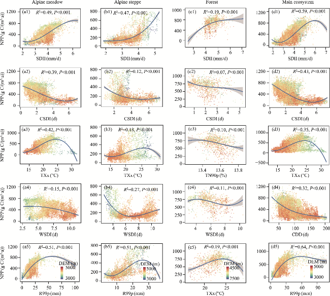
Fig. 9 Relationships between the NPP and extreme climate indices in the alpine meadow (a1-a5), alpine steppe (b1-b5), forest (c1-c5), and main ecosystem (d1-d5). The selection of extreme climate indices for different ecosystems is based on the mean absolute SHAP values. The DEM legend applies to all scatter plots within its respective column. The shaded area denotes the 95% confidence interval of the curve fitting.

4 Discussion

The NPP in different ecosystems across the QXP generally exhibited increasing trends from 1982 to 2020 (Fig. 5), which is consistent with the results of previous studies (Zhang et al., 2014; Shen et al., 2022b; Zhou et al., 2024). This phenomenon was closely linked to the impact of climate change. In recent decades, precipitation and temperature on the QXP have exhibited increasing trends (Yin et al., 2019; Ye et al., 2020). Existing studies have indicated that a favorable hydrothermal environment provides crucial conditions for vegetation growth (Frank et al., 2015). Adequate soil moisture ensures the normal operation of vegetation photosynthesis under appropriate CO2 concentration and light conditions (Gang et al., 2014; Ye et al., 2020). In addition, sufficient soil moisture ensures the absorption and transport of nutrients in vegetation (Sun et al., 2019). Hence, the increase in precipitation played an important role in the increase of NPP across the QXP. In addition to precipitation, temperature was another important climate factor influencing the increase in NPP. An increase in temperature can enhance the activity of photosynthetic enzymes (Sun et al., 2019). Furthermore, an increase in temperature facilitates the mineralization and decomposition of organic matter in the soil, thereby enhancing the absorption of the organic matter in the soil by vegetation (Melillo et al., 2002; Wan et al., 2005). In addition, the multi-year average NPP on the QXP exhibited strong spatial heterogeneity (Fig. 6). The reasons for this phenomenon are closely related to the unique climate and terrain of the QXP. The elevation of the QXP increases from southeast to northwest (Xu et al., 2023). Under the influences of the monsoon and elevation, precipitation and temperature on the QXP decreased from southeast to northwest (Ye et al., 2020). The unique spatial patterns of precipitation and temperature resulted in the forests mainly concentrated on the southeastern part of the QXP, while the alpine meadows and alpine steppes were distributed in the central and western regions of the QXP (Fig. 1). In addition, the snow-covered and desert areas were mainly concentrated on the northwestern part of the QXP due to the high elevation and harsh weather conditions. The total nitrogen content of the soil decreased with increasing elevation (Ye et al., 2020). These spatial variations will affect the normal physiological activities of vegetation. Overall, the unique hydrothermal pattern and soil trace element distribution across the QXP resulted in a decrease in NPP from southeast to northwest.
The results of this study indicated that the increases in R99p and SDII increased the NPP in different ecosystems on the QXP, while the increases in CSDI and WSDI decreased the NPP in these ecosystems. Similar results have been reported for the Yellow River Basin and Songhua River Basin in China (Xia et al., 2023; Cui et al., 2024). The differences in the impact mechanisms of extreme precipitation and extreme temperature on vegetation in different ecosystems and the adaptability of vegetation may lead to differences in the impact of extreme climate on NPP in different ecosystems (Li et al., 2019; Sun et al., 2019; Ye et al., 2020). Existing studies have shown that extreme climate events mainly have adverse effects on the structures and functions of terrestrial ecosystems (Piao et al., 2024). The vegetation on the QXP is primarily concentrated in the high-elevation areas with simple ecosystem structures. The aboveground parts of the terrestrial ecosystems will wither or even die under sustained low or high temperatures (Ye et al., 2020). According to related studies, in arid environments, plant growth, community structure, and ecosystem functions are generally limited by low precipitation availability (Niu et al., 2008; Winkler et al., 2016). Drought inhibits photosynthesis because soil moisture is a crucial intermediary for transport of nutrients in plants (Mäkiranta et al., 2017). In addition, water is necessary for the normal operation of vegetation photosynthesis (Ye et al., 2020). The increases in SDII and R99p can effectively alleviate the water shortage for vegetation, thereby improving the NPP across the QXP. In this study, we concluded that during the study period, the influence of extreme climate indices on NPP was greater than that of the length of vegetation growing season. Extreme climate events had a direct impact on the growth and survival conditions of vegetation and this impact was often direct and intense, potentially leading to damage to the physiological functions of vegetation (Allen et al., 2015). In contrast, the impact of the length of vegetation growing season on NPP was relatively small, mainly by affecting the physiological activity time of vegetation and thus affecting NPP.
In this study, the spatiotemporal patterns of NPP and the impact mechanisms of extreme climate and the length of vegetation growing season on NPP were analyzed. Nevertheless, this study has some limitations. First, many factors affect the NPP. Some changes in NPP are caused by climate factors, while other soil factors (i.e., soil moisture, soil temperature, and soil total potassium) have also been shown to affect the NPP (Ye et al., 2020). Hence, more attention should be paid to the relationships between the NPP and soil factors in future studies. Second, previous research has shown that extreme climate events often have lagged effects on NPP in different ecosystems (Wang and Rao, 2023). Therefore, it is necessary to explore the lag effect of extreme climate events on NPP at different time scales in future studies.

5 Conclusions

This study obtained a NDVI dataset (1982-2020) using a new data fusion method based on the MOD13A2 NDVI and GIMMS NDVI3g datasets and developed a NPP dataset across the QXP for the period 1982-2020. Besides, this study analyzed the spatiotemporal patterns of NPP and explored the impact mechanisms of extreme climate and the length of vegetation growing season on NPP. The results indicated that the simulated NDVI based on the new data fusion method and the estimated NPP based on the CASA model had good applicability. The NPP primarily exhibited an increasing trend in different ecosystems on the QXP. In addition, the NPP exhibited strong spatial heterogeneity. Finally, the impact of extreme climate on NPP was greater than that of the length of vegetation growing season. Among the extreme climate indices, the increases in R99p, SDII, and TXx increased the NPP in different ecosystems on the QXP, while the increases in CSDI and WSDI decreased the NPP in these ecosystems. The results of this study enhance our understanding of the sensitivity and vulnerability of ecosystems to extreme climate, providing a scientific basis for decision-making in response to extreme climate in different ecosystems on the QXP.

Conflict of interest

The authors declare that they have no known competing financial interests or personal relationships that could have appeared to influence the work reported in this paper.

Acknowledgements

This research was supported by the National Natural Science Foundation of China (U2243227).

Author contributions

Conceptualization: SUN Huaizhang; Methodology: SUN Huaizhang, LIU Jun; Formal analysis: SUN Huaizhang, ZHAO Xueqiang, CHEN Yangbo; Writing - original draft preparation: SUN Huaizhang; Writing - review and editing: SUN Huaizhang, ZHAO Xueqiang; Funding acquisition: CHEN Yangbo; Resources: SUN Huaizhang, LIU Jun; Supervision: CHEN Yangbo. All authors approved the manuscript.
[1]
Allen C D, Breshears D D, McDowell N G. 2015. On underestimation of global vulnerability to tree mortality and forest die-off from hotter drought in the Anthropocene. Ecosphere, 6(8): 129, doi: 10.1890/ES15-00203.1.

[2]
Breiman L. 2001. Random forests. Machine Learning, 45: 5-32.

[3]
Chen B X, Zhang X Z, Tao J, et al. 2014. The impact of climate change and anthropogenic activities on alpine grassland over the Qinghai-Tibet Plateau. Agricultural and Forest Meteorology, 189-190: 11-18.

[4]
Chen T, Xu Z W, Tang G P, et al. 2021. Spatiotemporal monitoring of soil CO2 efflux in a subtropical forest during the dry season based on field observations and remote sensing imagery. Remote Sensing, 13(17): 3481, doi: 10.3390/rs13173481.

[5]
Chen X Q, An S, Inouye D W, et al. 2015. Temperature and snowfall trigger alpine vegetation green-up on the world's roof. Global Change Biology, 21(10): 3635-3646.

[6]
Ciais P, Reichstein M, Viovy N, et al. 2005. Europe-wide reduction in primary productivity caused by the heat and drought in 2003. Nature, 437(7058): 529-533.

[7]
Clark D A, Brown S, Kicklighter D W, et al. 2001. Measuring net primary production in forests: Concepts and field methods. Ecological Applications, 11(2): 356-370.

[8]
Cui S, Jia Z Y, Guo L, et al. 2024. Impacts of extreme climate events at different altitudinal gradients on vegetation NPP in Songhua River Basin. Environmental Sciences, 45(1): 275-286. (in Chinese)

[9]
Cuo L, Zhang Y X, Xu R, et al. 2021. Decadal change and inter-annual variability of net primary productivity on the Tibetan Plateau. Climate Dynamics, 56(5-6): 1837-1857.

[10]
Dragoni D, Schmid H P, Wayson C A, et al. 2011. Evidence of increased net ecosystem productivity associated with a longer vegetated season in a deciduous forest in south-central Indiana, USA. Global Change Biology, 17(2): 886-897.

[11]
Frank D, Reichstein M, Bahn M, et al. 2015. Effects of climate extremes on the terrestrial carbon cycle: Concepts, processes and potential future impacts. Global Change Biology, 21(8): 2861-2880.

[12]
Gang C C, Zhou W, Chen Y Z, et al. 2014. Quantitative assessment of the contributions of climate change and human activities on global grassland degradation. Environmental Earth Sciences, 72(11): 4273-4282.

[13]
Gao Q Z, Wan Y F, Li Y, et al. 2012. Effects of topography and human activity on the net primary productivity (NPP) of alpine grassland in northern Tibet from 1981 to 2004. International Journal of Remote Sensing, 34(6): 2057-2069.

[14]
Ge W Y, Deng L Q, Wang F, et al. 2021. Quantifying the contributions of human activities and climate change to vegetation net primary productivity dynamics in China from 2001 to 2016. Science of the Total Environment, 773: 145648, doi: 10.1016/j.scitotenv.2021.145648.

[15]
He Y L, Yan W B, Cai Y, et al. 2022. How does the net primary productivity respond to the extreme climate under elevation constraints in mountainous areas of Yunnan, China? Ecological Indicators, 138: 108817, doi: 10.1016/j.ecolind.2022.108817.

[16]
Hou G Y, Wu S X, Long W Y, et al. 2023. Quantitative analysis of the impact of climate change and oasification on changes in net primary productivity variation in mid-Tianshan Mountains from 2001 to 2020. Ecological Indicators, 154: 110820, doi: 10.1016/j.ecolind.2023.110820.

[17]
Ji Z M, Kang S C, Cong Z Y, et al. 2015. Simulation of carbonaceous aerosols over the Third Pole and adjacent regions: distribution, transportation, deposition, and climatic effects. Climate Dynamics, 45(9-10): 2831-2846.

[18]
Jönsson P, Eklundh L. 2002. Seasonality extraction by function fitting to time-series of satellite sensor data. IEEE Transactions on Geoscience and Remote Sensing, 40(8): 1824-1832.

[19]
Jönsson P, Eklundh L. 2004. TIMESAT—a program for analyzing time-series of satellite sensor data. Computers & Geosciences, 30(8): 833-845.

[20]
Li C H, Sun H, Liu L H, et al. 2022. The importance of permafrost in the steady and fast increase in net primary production of the grassland on the Qinghai-Tibet Plateau. CATENA, 211(1): 105964, doi: 10.1016/j.catena.2021.105964.

[21]
Li C H, Liu Y F, Zhu T B, et al. 2023. Considering time-lag effects can improve the accuracy of NPP simulation using a light use efficiency model. Journal of Geographical Sciences, 33(5): 961-979.

[22]
Li H Y, Vulova S, Rocha A D, et al. 2024. Spatio-temporal feature attribution of European summer wildfires with Explainable Artificial Intelligence (XAI). Science of the Total Environment, 916: 170330, doi: 10.1016/j.scitotenv.2024.170330.

[23]
Li P, Liu Z L, Zhou X L, et al. 2021a. Combined control of multiple extreme climate stressors on autumn vegetation phenology on the Tibetan Plateau under past and future climate change. Agricultural and Forest Meteorology, 308-309: 108571, doi: 10.1016/j.agrformet.2021.108571.

[24]
Li X, Wu C F, Meadows M E, et al. 2021b. Factors underlying spatiotemporal variations in atmospheric PM2.5 concentrations in Zhejiang Province, China. Remote Sensing, 13(15): 3011, doi: 10.3390/rs13153011.

[25]
Li X Y, Li Y, Chen A P, et al. 2019. The impact of the 2009/2010 drought on vegetation growth and terrestrial carbon balance in Southwest China. Agricultural and Forest Meteorology, 269-270: 239-248.

[26]
Liu B, Guo H X, Li J L, et al. 2024. Application and interpretability of ensemble learning for landslide susceptibility mapping along the Three Gorges Reservoir area, China. Natural Hazards, 120(5): 4601-4632.

[27]
Liu D, Wang T, Yang T, et al. 2019a. Deciphering impacts of climate extremes on Tibetan grasslands in the last fifteen years. Science Bulletin, 64(7): 446-454.

[28]
Liu Y Y, Yang Y, Wang Q, et al. 2019b. Evaluating the responses of net primary productivity and carbon use efficiency of global grassland to climate variability along an aridity gradient. Science of the Total Environment, 652: 671-682.

[29]
Lundberg S M, Lee S I. 2017. A unified approach to interpreting model predictions. In:Proceedings of the 31st International Conference on Neural Information Processing Systems (NIPS'17). Curran Associates Inc., Red Hook, NY, USA, 4768-4777.

[30]
Mäkiranta P, Laiho R, Mehtätalo L, et al. 2017. Responses of phenology and biomass production of boreal fens to climate warming under different water-table level regimes. Global Change Biology, 24(3): 944-956.

[31]
Melillo J M, Steudler P A, Aber J D, et al. 2002. Soil warming and carbon-cycle feedbacks to the climate system. Science, 298(5601): 2173-2176.

[32]
Michaletz S T, Cheng D L, Kerkhoff A J, et al. 2014. Convergence of terrestrial plant production across global climate gradients. Nature, 512(7512): 39-43.

[33]
Niu S L, Wu M Y, Han Y, et al. 2008. Water-mediated responses of ecosystem carbon fluxes to climatic change in a temperate steppe. New Phytologist, 177(1): 209-219.

[34]
Piao S L, Friedlingstein P, Ciais P, et al. 2007. Growing season extension and its impact on terrestrial carbon cycle in the Northern Hemisphere over the past 2 decades. Global Biogeochemical Cycles, 21(3): GB3018, doi: 10.1029/2006GB002888.

[35]
Piao Z G, Li X Y, Xu H, et al. 2024. Threshold of climate extremes that impact vegetation productivity over the Tibetan Plateau. Science China Earth Sciences, 67: 1967-1977.

[36]
Prăvălie R, Niculiță M, Roșca B, et al. 2023. Machine learning-based prediction and assessment of recent dynamics of forest net primary productivity in Romania. Journal of Environmental Management, 334: 117513, doi: 10.1016/j.jenvman.2023.117513.

[37]
Sen P K. 1968. Estimates of the regression coefficient based on Kendall's Tau. Journal of the American Statistical Association, 63(324): 1379-1389.

[38]
Shen M G, Wang S P, Jiang N, et al. 2022a. Plant phenology changes and drivers on the Qinghai-Tibetan Plateau. Nature Reviews Earth & Environment, 3(10): 633-651.

[39]
Shen X J, Liu Y W, Zhang J Q, et al. 2022b. Asymmetric impacts of diurnal warming on vegetation carbon sequestration of marshes in the Qinghai Tibet Plateau. Global Biogeochemical Cycles, 36(7): e2022GB007396, doi: 10.1029/2022GB007396.

[40]
Sun J, Zhou T C, Liu M, et al. 2019. Water and heat availability are drivers of the aboveground plant carbon accumulation rate in alpine grasslands on the Tibetan Plateau. Global Ecology and Biogeography, 29(1): 50-64.

[41]
Sun J, Ye C C, Liu M, et al. 2022. Response of net reduction rate in vegetation carbon uptake to climate change across a unique gradient zone on the Tibetan Plateau. Environmental Research, 203: 111894, doi: 10.1016/j.envres.2021.111894.

[42]
Wan S Q, Hui D F, Wallace L, et al. 2005. Direct and indirect effects of experimental warming on ecosystem carbon processes in a tallgrass prairie. Global Biogeochemical Cycles, 19(2): GB2014, doi: 10.1029/2004GB002315.

[43]
Wang F E, Wang Y X, Zhang K, et al. 2021. Spatial heterogeneity modeling of water quality based on random forest regression and model interpretation. Environmental Research, 202: 111660, doi: 10.1016/j.envres.2021.111660.

[44]
Wang H, Yan S J, Ciais P, et al. 2022. Exploring complex water stress-gross primary production relationships: Impact of climatic drivers, main effects, and interactive effects. Global Change Biology, 28(13): 4110-4123.

[45]
Wang M M, Wang S Q, Wang J B, et al. 2018. Detection of positive gross primary production extremes in terrestrial ecosystems of China during 1982-2015 and analysis of climate contribution. Journal of Geophysical Research: Biogeosciences, 123(9): 2807-2823.

[46]
Wang Y E, Rao L Y. 2023. Impact of climatic factors and human activities on the net primary productivity of the vegetation in the Pisha sandstone area. Arid Zone Research, 40(12): 1982-1995. (in Chinese)

[47]
Wei X D, Yang J, Luo P P, et al. 2022. Assessment of the variation and influencing factors of vegetation NPP and carbon sink capacity under different natural conditions. Ecological Indicators, 138: 108834, doi: 10.1016/j.ecolind.2022.108834.

[48]
Winkler D E, Chapin K J, Kueppers L M. 2016. Soil moisture mediates alpine life form and community productivity responses to warming. Ecology, 97(6): 1553-1563.

[49]
Xia B, Ma P Y, Xu C, et al. 2023. Spatiotemporal variation of NPP and its response to extreme climate indices in Yellow River Basin in recent 20 years. Research of Soil and Water Conservation, 30(2): 256-266. (in Chinese)

[50]
Xu B N, Li J J, Pei X J, et al. 2023. Decoupling the response of vegetation dynamics to asymmetric warming over the Qinghai-Tibet plateau from 2001 to 2020. Journal of Environmental Management, 347: 119131, doi: 10.1016/j.jenvman.2023.119131.

[51]
Xu Y Q, Xiao F J, Yu L. 2020. Review of spatio-temporal distribution of net primary productity in forest ecosystem and its responses to climate change in China. Acta Ecologica Sinica, 40(14): 4710-4723. (in Chinese)

[52]
Xue Y Y, Bai X Y, Zhao C W, et al. 2023. Spring photosynthetic phenology of Chinese vegetation in response to climate change and its impact on net primary productivity. Agricultural and Forest Meteorology, 342: 109734, doi: 10.1016/j.agrformet.2023.109734.

[53]
Yan Y C, Liu X P, Ou J P, et al. 2018. Assimilating multi-source remotely sensed data into a light use efficiency model for net primary productivity estimation. International Journal of Applied Earth Observation and Geoinformation, 72: 11-25.

[54]
Yang H F, Zhong X N, Deng S Q, et al. 2021. Assessment of the impact of LUCC on NPP and its influencing factors in the Yangtze River basin, China. CATENA, 206: 105542, doi: 10.1016/j.catena.2021.105542.

[55]
Ye C C, Sun J, Liu M, et al. 2020. Concurrent and lagged effects of extreme drought induce net reduction in vegetation carbon uptake on Tibetan Plateau. Remote Sensing, 12(15): 2347, doi: 10.3390/rs12152347.

[56]
Yin H, Sun Y, Donat M G. 2019. Changes in temperature extremes on the Tibetan Plateau and their attribution. Environmental Research Letters, 14(12): 124015, doi: 10.1088/1748-9326/ab503c.

[57]
Yin S Y, Du H Q, Mao F J, et al. 2024. Spatiotemporal patterns of net primary productivity of subtropical forests in China and its response to drought. Science of the Total Environment, 913: 169439, doi: 10.1016/j.scitotenv.2023.169439.

[58]
Yong Z Y, Xiong J N, Wang Z G, et al. 2021. Relationship of extreme precipitation, surface air temperature, and dew point temperature across the Tibetan Plateau. Climatic Change, 165(1-2): 41, doi: 10.1007/s10584-021-03076-2.

[59]
Zhang G L, Xu X L, Zhou C P, et al. 2011a. Responses of grassland vegetation to climatic variations on different temporal scales in Hulun Buir Grassland in the past 30 years. Journal of Geographical Sciences, 21(4): 634-650.

[60]
Zhang X B, Alexander L, Hegerl C C, et al. 2011b. Indices for monitoring changes in extremes based on daily temperature and precipitation data. Wiley Interdisciplinary Reviews: Climate Change, 2(6): 851-870.

[61]
Zhang Y L, Qi W, Zhou C P, et al. 2014. Spatial and temporal variability in the net primary production of alpine grassland on the Tibetan Plateau since 1982. Journal of Geographical Sciences, 24(2): 269-287.

[62]
Zhou W, Wang T, Xiao J Y, et al. 2024. Grassland productivity increase was dominated by climate in Qinghai-Tibet Plateau from 1982 to 2020. Journal of Cleaner Production, 434(3): 140144, doi: 10.1016/j.jclepro.2023.140144.

[63]
Zhu Y H, Luo P P, Zhang S, et al. 2020. Spatiotemporal analysis of hydrological variations and their impacts on vegetation in semiarid areas from multiple satellite data. Remote Sensing, 12(24): 4177, doi: 10.3390/rs12244177.

文章导航

/