
Impact of urban sprawl on land surface temperature in the Mashhad City, Iran: A deep learning and cloud- based remote sensing analysis
Received date: 2024-09-19
Revised date: 2025-01-14
Accepted date: 2025-01-25
Online published: 2025-08-13
Komeh ZINAT , Hamzeh SAEID , Memarian HADI , Attarchi SARA , LU Linlin , Naboureh AMIN , Alavipanah KAZEM SEYED . [J]. Journal of Arid Land, 2025 , 17(3) : 285 -303 . DOI: 10.1007/s40333-025-0009-7
The evolution of land use patterns and the emergence of urban heat islands (UHI) over time are critical issues in city development strategies. This study aims to establish a model that maps the correlation between changes in land use and land surface temperature (LST) in the Mashhad City, northeastern Iran. Employing the Google Earth Engine (GEE) platform, we calculated the LST and extracted land use maps from 1985 to 2020. The convolutional neural network (CNN) approach was utilized to deeply explore the relationship between the LST and land use. The obtained results were compared with the standard machine learning (ML) methods such as support vector machine (SVM), random forest (RF), and linear regression. The results revealed a 1.00°C-2.00°C increase in the LST across various land use categories. This variation in temperature increases across different land use types suggested that, in addition to global warming and climatic changes, temperature rise was strongly influenced by land use changes. The LST surge in built-up lands in the Mashhad City was estimated to be 1.75°C, while forest lands experienced the smallest increase of 1.19°C. The developed CNN demonstrated an overall prediction accuracy of 91.60%, significantly outperforming linear regression and standard ML methods, due to the ability to extract higher level features. Furthermore, the deep neural network (DNN) modeling indicated that the urban lands, comprising 69.57% and 71.34% of the studied area, were projected to experience extreme temperatures above 41.00°C and 42.00°C in the years 2025 and 2030, respectively. In conclusion, the LST predictioin framework, combining the GEE platform and CNN method, provided an effective approach to inform urban planning and to mitigate the impacts of UHI.
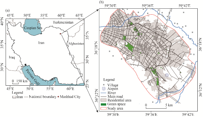
Fig. 1 Geographical location of the Mashhad City (a), Iran and the overview of the city (b) |
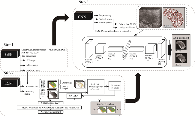
Fig. 2 Data processing framework of the study. GEE, Google Earth Engine; TM, thematic mapper; ETM, enhanced thematic mapper; OLI, operational land imager; LCM, land change modeler; CA-ANN, cellular automata-artificial neural network; CONV, convolutional layer. |
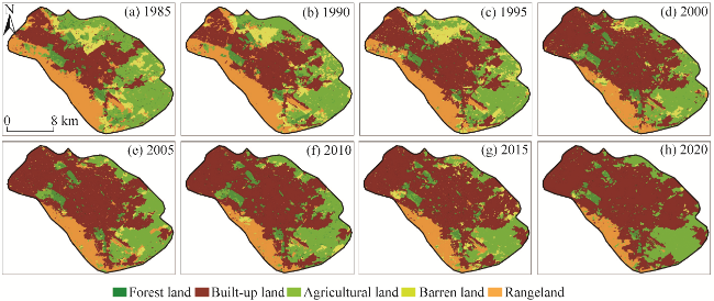
Fig. 3 Changes of different land use types of the Mashhad City from 1985 to 2020. (a), 1985; (b), 1990; (c), 1995; (d), 2000; (e), 2005; (f), 2010; (g), 2015; (h), 2020. |
Table 1 Accuracy measurement for the generated land use dataset |
| Accuracy | 1985 | 1990 | 1995 | 2000 | 2005 | 2010 | 2015 | 2020 |
|---|---|---|---|---|---|---|---|---|
| Overall accuracy (%) | 92.70 | 89.40 | 91.00 | 91.20 | 91.90 | 91.00 | 96.90 | 94.00 |
| PA (%) | 90.00 | 87.60 | 91.40 | 86.80 | 92.60 | 92.40 | 96.60 | 93.60 |
| UA (%) | 88.60 | 90.00 | 91.00 | 89.60 | 92.60 | 91.00 | 96.60 | 94.20 |
Note: PA, producer accuracy; UA, user accuracy. |
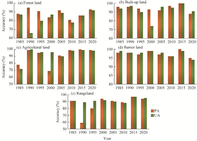
Fig. 4 Producer accuracy (PA) and user accuracy (UA) metrics for different land use types from 1985 to 2020. (a), forest land, (b), built-up land; (c), agricultural land; (d), barren land; (e), rangeland. |
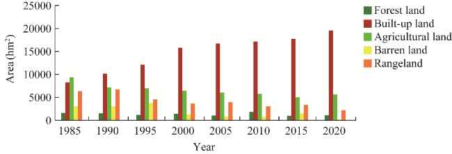
Fig. 5 Area changes of different land use types of the Mashhad City from 1985 to 2020 |
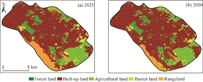
Fig. 6 Projected map of different land use types in the years 2025 (a) and 2030 (b) |
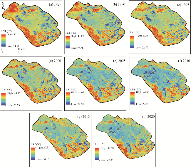
Fig. 7 Land surface temperature (LST) maps of the Mashhad City from 1985 to 2020. (a), 1985; (b), 1990; (c), 1995; (d), 2000; (e), 2005; (f), 2010; (g), 2015; (h), 2020. |
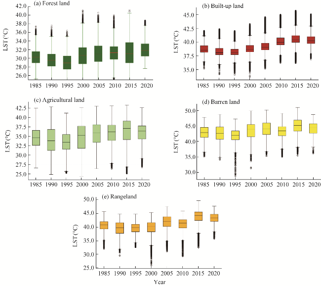
Fig. 8 Box plots of LST for different land use types from 1985 to 2020. (a), forest land; (b), built-up land; (c), agricultural land; (d), barren land; (e), rangeland. Boxes indicate the IQR (interquartile range, 75th to 25th of the data). The median value is shown as a line within the box. Outlier is shown as black circle. Bars extend to the most extreme value within 1.5×IQR. |
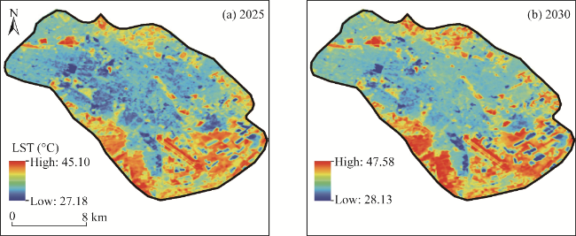
Fig. 9 LST maps simulated using the convolutional neural network (CNN) in the years 2025 (a) and 2030 (b) |
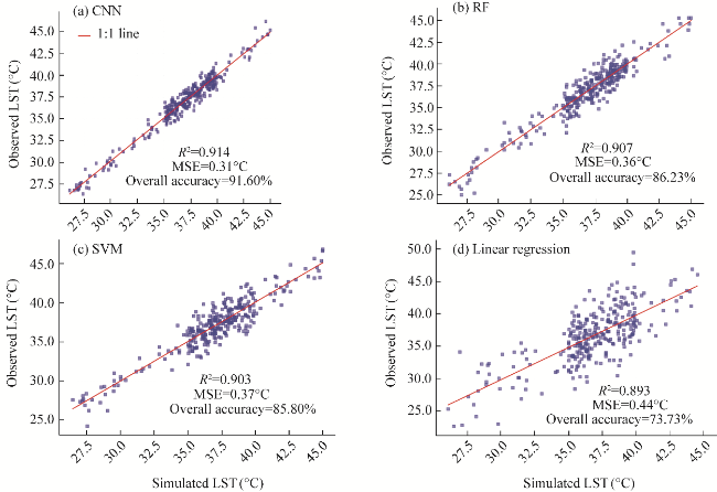
Fig. 10 Correlation between simulated and observed LST for the year 2020 using four different methods. (a), CNN; (b), random forest (RF); (c), support vector machine (SVM); (d), linear regression. R2, determination of coefficient; MSE, mean squared error. |
| [1] |
|
| [2] |
|
| [3] |
|
| [4] |
|
| [5] |
|
| [6] |
|
| [7] |
|
| [8] |
|
| [9] |
|
| [10] |
|
| [11] |
|
| [12] |
|
| [13] |
|
| [14] |
|
| [15] |
|
| [16] |
|
| [17] |
|
| [18] |
|
| [19] |
|
| [20] |
|
| [21] |
|
| [22] |
|
| [23] |
|
| [24] |
|
| [25] |
|
| [26] |
|
| [27] |
|
| [28] |
|
| [29] |
|
| [30] |
|
| [31] |
|
| [32] |
|
| [33] |
IPCC (Intergovernmental Panel on Climate Change). 2014. Mitigation of climate change. Contribution of working group III to the fifth assessment report of the intergovernmental panel on climate change, 1454: 147, doi: 10.1017/CBO9781107415416.
|
| [34] |
|
| [35] |
|
| [36] |
|
| [37] |
|
| [38] |
|
| [39] |
|
| [40] |
|
| [41] |
|
| [42] |
|
| [43] |
|
| [44] |
|
| [45] |
|
| [46] |
|
| [47] |
|
| [48] |
|
| [49] |
|
| [50] |
|
| [51] |
|
| [52] |
|
| [53] |
|
| [54] |
|
| [55] |
|
| [56] |
|
| [57] |
|
| [58] |
|
| [59] |
|
| [60] |
|
| [61] |
|
| [62] |
|
| [63] |
|
| [64] |
|
| [65] |
|
| [66] |
|
| [67] |
|
| [68] |
|
| [69] |
|
| [70] |
|
| [71] |
|
| [72] |
|
| [73] |
|
| [74] |
|
| [75] |
|
| [76] |
|
| [77] |
|
| [78] |
|
| [79] |
|
| [80] |
|
| [81] |
|
| [82] |
|
| [83] |
|
| [84] |
|
| [85] |
|
| [86] |
|
| [87] |
|
| [88] |
|
| [89] |
|
| [90] |
|
/
| 〈 |
|
〉 |