• Suzan ISMAIL , * ,
  • Hamid MALIKI
展开

收稿日期: 2024-04-13

  修回日期: 2024-07-26

  录用日期: 2024-08-13

  网络出版日期: 2025-08-13

Spatiotemporal landscape pattern changes and their effects on land surface temperature in greenbelt with semi-arid climate: A case study of the Erbil City, Iraq

  • Suzan ISMAIL , * ,
  • Hamid MALIKI
Expand
  • Department of Architecture, College of Engineering, Salahaddin University, Erbil 44002, Iraq
*Suzan ISMAIL (E-mail: )

Received date: 2024-04-13

  Revised date: 2024-07-26

  Accepted date: 2024-08-13

  Online published: 2025-08-13

本文引用格式

Suzan ISMAIL , Hamid MALIKI . [J]. Journal of Arid Land, 2024 , 16(9) : 1214 -1231 . DOI: 10.1007/s40333-024-0027-x

Abstract

Urban expansion of cities has caused changes in land use and land cover (LULC) in addition to transformations in the spatial characteristics of landscape structure. These alterations have generated heat islands and rise of land surface temperature (LST), which consequently have caused a variety of environmental issues and threated the sustainable development of urban areas. Greenbelts are employed as an urban planning containment policy to regulate urban expansion, safeguard natural open spaces, and serve adaptation and mitigation functions. And they are regarded as a powerful measure for enhancing urban environmental sustainability. Despite the fact that, the relation between landscape structure change and variation of LST has been examined thoroughly in many studies, but there is a limitation concerning this relation in semi-arid climate and in greenbelts as well, with the lacking of comprehensive research combing both aspects. Accordingly, this study investigated the spatiotemporal changes of landscape pattern of LULC and their relationship with variation of LST within an inner greenbelt in the semi-arid Erbil City of northern Iraq. The study utilized remote sensing data to retrieve LST, classified LULC, and calculated landscape metrics for analyzing spatial changes during the study period. The results indicated that both composition and configuration of LULC had an impact on the variation of LST in the study area. The Pearson's correlation showed the significant effect of Vegetation 1 type (VH), cultivated land (CU), and bare soil (BS) on LST, as increase of LST was related to the decrease of VH and the increases of CU and BS, while, neither Vegetation 2 type (VL) nor built-up (BU) had any effects. Additionally, the spatial distribution of LULC also exhibited significant effects on LST, as LST was strongly correlated with landscape indices for VH, CU, and BS. However, for BU, only aggregation index metric affected LST, while none of VL metrics had a relation. The study provides insights for landscape planners and policymakers to not only develop more green spaces in greenbelt but also optimize the spatial landscape patterns to reduce the influence of LST on the urban environment, and further promote sustainable development and enhance well-being in the cities with semi-arid climate.

1 Introduction

In recent decades, the topic of urbanization and its effects on the environment has gained world-wide recognition and concern, owing to the substantial influence on global environment. The expansion of urban areas within cities can lead to significant alterations in land use and land cover (LULC), which is a vital factor in regional and global climate change, thus affecting local ecosystems and people well-being (Rimal et al., 2019). The process of urban land expansion is directly associated with the decrease in natural vegetation and the subsequent rise in man-made surfaces in the surrounding areas of cities (Abebe et al., 2022). The deterioration of landscape, deforestation, soil loss, and the destruction of natural habitats are the main consequences of changes in LULC. On a regional level, transition from greenery to built-up areas modifies the local climate and can result in changes in local atmosphere (Senanayake et al., 2013). Furthermore, variations in thermal conditions, like the formation of heat islands and alteration of land surface temperature (LST), represent additional outcomes resulting from significant modifications in surface cover (Kumari and Sarma, 2017; Bhagat and Prasad, 2023). For instance, when forest cover is removed and replaced, LST increases due to alterations in the physical qualities of the land surface (Debie et al., 2022). Likewise, raised LST in cities leads to negative implications such as anthropogenic production of heat, decreased air quality from increased emission of greenhouse gas, and air contaminant (Balany et al., 2020). All of the above have led to a range of environmental issues, hence posing a threat to the sustainable development of urban areas and its environment.
Green spaces play a crucial role in the regulation of urban thermal environment and the enhancement of local microclimate within urban areas. They have the capacity to modulate air flow and heat exchange in order to produce cooling island effects through evapotranspiration and emissivity, in conjunction with reduced thermal inertia (Li and Zhou, 2019). Consequently, green spaces have been found to be the most efficient kind of land cover in minimizing the impacts of urban heat islands (UHIs) and decreasing LST. Urban areas, on the other hand, are able to absorb and transform a greater amount of solar radiation to thermal energy because their impermeable surfaces typically contain both heat-absorbing and heat-reflecting elements (Galvez et al., 2024).
Thus, planners and policymakers have adopted diverse urban containment strategies to regulate the urban expansion, safeguard green spaces, and influence the spatial development of urban areas (Bengston and Youn, 2006). Among various planning management policies, greenbelts are considered as the most common strategies for managing urban development. They are development-restricted zones established with the goal of minimizing urban sprawl and creating a healthy living environment for inhabitants by conserving natural environment that surrounds cities. Amati (2016) states that greenbelts are an important tool for protecting the environment, creating open space, controlling excessive urban growth, and ensuring the sustainability of larger green spaces around urban areas. In the 21st century, the urgency to minimize sprawl is reinforced by the prominent issues of climate change and sustainability as greenbelts could provide ecological restoration, mitigate UHIs effects, and affect climate change. As a result, under these conditions, greenbelts serve a variety of adaptation and mitigation functions, and they are regarded as a powerful measure for enhancing urban environmental sustainability (Han et al., 2017). The objectives of these greenbelts studies were to manage LULC changes, create and protect green surfaces in greenbelts primarily by scale and proportion, and therefore decrease the effect of urbanization on the landscape.
Human activities, on the other hand, not only caused changes in LULC, but also significantly contributed to variations in the spatial aspects of landscape structure (Wang et al., 2023). Landscape ecology is one field that seeks to understand and enhance the interdependence of landscape patterns with ecological processes (Turner, 2005). Within landscape ecology, landscape pattern study centers on the quantification and analysis of alterations in the compositions and configurations of land features using landscape metrics (Fan and Myint, 2014). The metrics are considered to be essential tools for comprehending the structure, function, and changes in landscape (O'Neill et al., 1988). Humans are a crucial part in landscape formation, as their land use practices have a major impact on the structure and function of landscape. Landscape ecology offers a comprehensive method for examining how changes in environmental conditions resulting from human land use activities are connected to landscape patterns (Abdullah and Nakagoshi, 2006). For instance, the increase in surface temperature caused by landscape pattern alterations can result in numerous ecological consequences, creating harmful impacts on the sustainable environment (Jia et al., 2022). Hence, recognizing the connections between land use and landscape pattern, as well as urban planning policy for land development, is essential for enhancing the environmental sustainability (Abdullah and Nakagoshi, 2006).
Recent advancement in remote sensing techniques and the availability of free time series data have provided essential knowledge and instrument for studying changes in LULC and landscape pattern. Furthermore, the thermal data in satellite images serve as the foundation for calculating LST, which can be valuable for environmental and climate change research in urban areas through the examination of UHIs to detect alterations in the landscape (Quattrochi and Luvall, 2014). Thus, scholars have conducted intensive research on the relation of landscape pattern with LST, as the influence of landscape composition and configuration on LST has been thoroughly explored across many climatic situations (Connors et al., 2013; Estoque et al., 2017; Amani-Beni et al., 2019; Effati et al., 2021). In general, the mentioned studies indicated that landscape pattern metrics can efficiently explicate LST in urban settings across diverse climates. Nevertheless, in certain cases, studies have shown conflicting outcomes. For instance, shape mean index that measures shape complexity, was found to have a negative correlation with LST in green areas with trees, in Accra, a tropical sub-Saharan city, Ghana (Athukorala and Murayama, 2020). On the other hand, in Beijing, China, a city with a monsoon-influenced humid continental climate, the metrics showed a positive correlation (Liu et al., 2022b). In a research done by Azhdari et al. (2018) in Shiraz City, Iran, which has a semi-arid climate, the influence of landscape structure and urban form on LST was investigated. The study found a positive correlation between landscape shape index (LSI) and LST for built-up land. On the contrary, a research conducted by Li et al. (2012) in Beijing City found a positive association between LSI for green space and LST. The same finding was also observed in Hangzhou City, China, which is characterized by a monsoon climate (Song et al., 2020). The largest patch index (LPI), a landscape metric that represents dominance, exhibited a negative correlation with LST in green space of Hangzhou City (Song et al., 2020), Fuzhou City (Liu et al., 2022a) in China, and Accra City in Ghana (Athukorala and Murayama, 2020). These areas have monsoon, subtropical marine monsoon, and tropical sub-Saharan climates, respectively. However, in Beijing City, LPI showed a positive correlation (Li et al., 2013b).
These findings indicated that a particular landscape metric may have varying uses, and some may even have opposite impacts on the thermal environment. Previous studies attribute these variations to the diverse climatic conditions in the study areas (Zhou et al., 2017). Thus, the utilization of research findings for the purpose of urban planning implications is limited by the difference in results. Hence, performing more study is vital to effectively develop and manage urban landscape areas in various climatic situations. Nevertheless, there is a constraint on research conducted in arid and semi-arid areas. In a systematic review conducted by Li et al. (2023) on the significance of landscape metrics in evaluating how the configuration of urban green spaces influences LST to detect their cooling effect. They reviewed 167 studies based on their climate zones and countries. The findings indicated that there were significantly less studies conducted in the arid climatic area compared with other climate areas. Additionally, there was a complete absence of research on this issue in Iraq, highlighting the urgent need for more studies in the arid areas and to address the knowledge gap in Iraq.
Prior studies have thoroughly stated the importance of greenbelts' impacts for urban development. Han et al. (2017) analyzed the impact of greenbelts deregulation on urban land growth in Seoul City, South Korea, revealing differences in land use expansion. Another study investigated Shanghai City in China to understand the influence of land use, land cover, and socioeconomic factors on the evolution of greenbelts (Wang et al., 2014). Likewise, the spatial and temporal variations of greenbelts in Beijing City, China were analyzed by utilizing remote sensing data (Yang and Jin, 2007). The aforementioned studies have investigated the impacts of greenbelts on urbanization and land development. Additionally, previous studies of greenbelts were also concerned to link land use change with environmental factors such as LST, carbon dioxide (CO2) emissions, and air pollution. A research in the United States evaluated the effectiveness of greenbelts in six counties for controlling urban expansion and preserving open land. The result found that the priority of land uses should be conserved and safeguarded in these greenbelts (Han et al., 2022). Another study conducted by Kardani-Yazd et al. (2019) examined the planning of urban greenbelts in Mashh City, Iran. The study utilized the environmental change index to evaluate the sensitivity and environmental modifications in greenbelts. In summary, the mentioned studies on greenbelts have demonstrated that greenbelts have a beneficial role in managing urban expansion and changes in land use, and preserving the quality of urban environments.
Ultimately, from what has been mentioned, it can be concluded that, although, the relation of landscape spatial characteristics with LST in general has been mentioned thoroughly, but there is a limitation in literature concerning this relation in the semi-arid climate and in the greenbelts as well, with the lacking of comprehensive research combing both aspects. Taking the greenbelt of the Erbil City with semi-arid climate, as the study area, this research investigated the spatiotemporal changes of landscape pattern of LULC and their relationship with LST. More specific aims are to: (1) quantify the spatial and temporal variations of LULC in greenbelt in the Erbil City; (2) assess the spatial and temporal changes of LST; (3) analyze the impact of LULC changes on LST; (4) determine the relation between changes in landscape pattern and LST; and (5) identify the primary spatial metrics that influence LST through landscape characteristics. The study provides urban planners and policymakers with deep insights to make decisions about reducing LST effects through the landscape spatial pattern of LULC in greenbelt to further promote sustainable development and enhance well-being.

2 Materials and methods

2.1 Study area

Erbil, the fourth largest city situated in northern Iraq, serves as the capital of the Kurdistan Region (36°06ʹ54ʺ-36°16ʹ45ʺN, 43°55ʹ15ʺ-44°05ʹ31ʺE). It has a semi-arid continental climate with dry and warm summers, and rainy and chilly winters. The lowest temperature was 6.20°C in January, while the highest temperature was 42.70°C in July in 2021. The maximum precipitation was 91.70 mm in December and the minimum precipitation was 0.00 mm in June (https://krso.gov.krd/en/statistics/environment).
The city has experienced significant economic growth since 2003 (Baper et al., 2013), resulting in rapid expansion of urban areas, which had an effect on the wide green spaces surrounding the city. The Erbil Inner Greenbelt (EIGB) as a key project was put forth in the City Master Plan of 2007. The project was approved on 9 January, 2013, with the goal of regulating urban growth and ensuring the survival of bigger green spaces near the Erbil City. According to the City Master Plan of 2007, the EIGB spans 12.00 km from the center of the Erbil City and is bounded by Ring Ways 8 and 9. It is located in the city's surroundings, outside the urbanized areas, and has a width of 2.00 km with an area of 164.75 km2. Regarding the vegetation present in the study area, it is composed of shrubs, crops, and grains with small patches of trees, while, the grass occupies the largest area portion within vegetation cover.

2.2 Data sources and preprocessing

Two Landsat satellite images retrieved from the United States Geological Survey (USGS) Earth Explorer website (https://earthexplorer.usgs.gov/) were utilized as the primary data in the study: Landsat-7 on 16 April, 2000 and Landsat-8 on 21 April, 2022 (Table 1). The remotely sensed datasets used a variety of sensors, including the L7 enhanced thematic mapper plus (ETM+) and L8 operational land imager (OLI) along with the thermal infrared sensor (TIRS) with 30 m spatial resolution. The data type of images had relatively cloud-free scenes, with a cloud cover of 2.00% for L7 and 0.14% for L8. The images are associated with a path/row combination, namely 169/35. With a gap of 22, the years 2000 and 2022 were chosen to detect the changes in the study area before the approval of EIGB, in 2013, and afterwards. The acquisition of the images took place in April, as the study area experienced the highest amount of vegetation growth during this period (Gaznayee et al., 2022). In addition, secondary data and materials were used in this study comprising of the map of EIGB, Erbil Master Plan of 2007, the geometrically corrected map of the Erbil City, and the map of the Erbil City with a high resolution. Furthermore, the study used high-resolution maps obtained from Google Earth Pro as part of its dataset.
Table 1 Satellite images and descriptions
Satellite/Sensor Landsat-7 ETM+ Landsat-8 OLI TIRS
Image ID LE07_L1TP_169035_20000416_20200918_02_T1 LC08_L1TP_169035_20220421_
20220428_02_T1
Path/Row 169/35 169/35
Date acquired (dd/mm/yyyy) 16/04/2000 21/04/2022
Scene center time 07:31:00 AM (LST) 07:38:00 AM (LST)
Cloud cover (%) 0.00 0.14
Projection UTM Zone 38 UTM Zone 38
Ellipsoid WGS 84 WGS 84
Resolution (m) 30 30

Note: ETM+, enhanced thematic mapper plus; OLI, operational land imager; TIRS, thermal infrared sensor; ID, identification card; UTM, universal transverse Mercator; AM, ante meridiem; WGS 84, world geodetic system 1984. The images are cited from the website of https://earthexplorer.usgs.gov/.

Following the download of satellite images and in order to prepare the images for spatiotemporal analysis, it was vital that preprocessing should be conducted, since the data of Landsat 7 and 8 are Level 1 products (Fig. 1). Preprocessing comprises geometric and atmospheric corrections that reduce various instrumental errors, noise from different sources, as well as lens distortions present in the photos (Moravec et al., 2021).
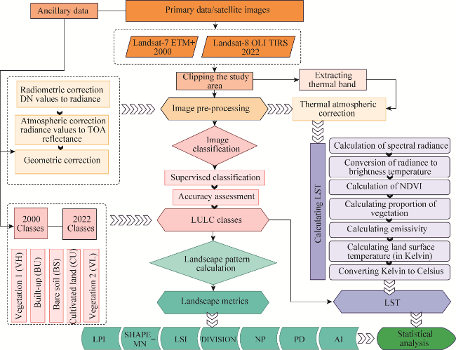
Fig. 1 Flowchart of the methodology used in the study. DN, digital number; TOA, top of atmosphere; LULC, land use and land cover; NDVI, normalized difference vegetation index; LST, land surface temperature; LPI, largest patch index; SHAPE_MN, mean shape index; LSI, landscape shape index; DIVISION, landscape division index; NP, number of patches; PD, patch density; AI, aggregation index. The abbreviations are the same in the following figures.
Initially, in order to perform atmospheric correction, the images undertook a correction process in which the digital numbers were transformed into radiance values. This transformation was achieved by utilizing the relevant information contained in their metadata files. Subsequently, the resulting images undertook a conversion process as the radiance values were converted into top-of-atmosphere reflectance. This conversion was carried out with the fast line-of-sight atmospheric analysis of hpercubes (FLAASH) module within ENVI v.5.3 software. On the other hand, before land surface temperature calculations could be determined, the thermal atmospheric correction technique in Envi software was utilized to correct the thermal infrared bands in Landsats 7 and 8. After the appropriate atmospheric adjustments have been made and temporal variations was dealt, proper pixel alignment in the chosen photos was critical (Liang and Wang, 2019). As a result, a procedure of an image-to-image registration method was implemented, in which the selected research image was made to correspond to another accurately adjusted image of the study area. A selection of ground control points in 2000 and 2022 was used with root mean square errors (RMSE) of 0.28 and 0.26, respectively.

2.3 Image processing and data analysis

2.3.1 LULC classification

Two satellite images in 2000 and 2022 were divided into five distinct types (Fig. 2), which were built-up (BU), bare soil (BS), cultivated land (CU), vegetation 1 (VH), and vegetation 2 (VL) (Table 2). VH includes many life forms of plant such as crops, grains, shrubs, and dispersed trees, while VL primarily comprises grasslands (Anderson et al., 1976). In addition, supplementary data obtained from Google Earth Pro and high-resolution images of the Erbil City have been used throughout the procedure. The evaluation of the classification's accuracy was carried out using a confusion matrix (Ali and Johnson, 2022). The assessment results indicate that the overall accuracies of classification in 2000 and 2022 were 92.00% and 94.60%, respectively.
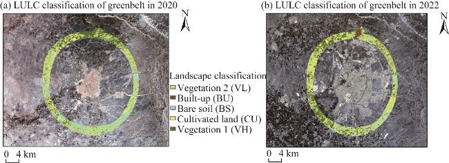
Fig. 2 LULC classification of greenbelt in 2000 (a) and 2022 (b)
Table 2 LULC classification of greenbelt and description
LULC classification Description
Built-up (BU) Settlements like built up village lands, roadways, and dispersed residential areas
Bare soil (BS) Areas characterized by the absence of vegetation with surface comprising of rock, sand, or clay
Cultivated land (CU) Areas specifically prepared for agricultural use
Vegetation 1 (VH) Many life forms of plant including crops, grains, shrubs, and dispersed trees
Vegetation 2 (VL) Areas primarily comprise grasslands
Additionally, the Kappa coefficient was found to be 0.90 and 0.93, correspondingly (Table 3). The research area's images were divided into polygon grids using ArcGIS v.10.8.1. This was achieved by generating a fishnet with dimensions of 0.9 km×0.9 km. Subsequently, a random sampling approach was employed to select 136 samples out of a total of 205 for each year. The extraction of the data was conducted in order to calculate landscape pattern at the class-level spatial metrics using Fragstats v.4.2 software.
Table 3 Accuracy of classification of LULC of greenbelt in 2000 and 2022
Year Accuracy BU BS CU VH VL OA KC
(%)
2000 UA 90.00 90.00 96.66 90.00 93.33 92.00 0.90
PA 87.09 84.37 93.54 100.00 96.55 - -
2022 UA 90.00 93.33 93.33 100.00 96.66 94.66 0.93
PA 96.42 87.50 93.33 100.00 96.66 - -

Note: UA, user's accuracy; PA, producer's accuracy; OA, overall accuracy; KC, Kapa coefficient; -, no value.

2.3.2 Landscape metrics

Landscape metrics are used as valuable tools for quantifying the spatial attributes of diverse LULC categories. The metrics function as indicator of landscape pattern composition and configuration, and is used in the assessment of both spatial and temporal variations in landscape (McGarigal and Marks, 1995). The concept of landscape composition focuses on the characteristics related to the occurrence and proportion of different land cover types, without clearly defining their spatial characteristics. Landscape configuration, conversely, refers to the spatial organization and distribution of the patches existing within the landscape (Vanderhaegen and Canters, 2010). Landscape metrics can be computed at both the class and the landscape levels. Class level metrics are beneficial for studying landscape development, as they indicate the spatial distribution and patterns in the landscape of a specific land cover type.
This study examined several landscape measures based on their significance in the literature and prior studies. Following that, we selected seven metrics at the class level in accordance with the study's objectives. These metrics are commonly used for evaluating the relationship between patterns of landscape and LST (Estoque et al., 2017; Yang et al., 2017). The selected metrics include the largest patch index (LPI), mean shape index (SHAPE_MN), landscape shape index (LSI), division index (DIVISION), aggregation index (AI), number of patches (NP), and patch density (PD) (Mcgarigal, 2014; Song et al., 2020; Table 4).
Table 4 Landscape metrics of greenbelt for the study
Landscape metric Abbreviation Description Category Unit Range
Largest patch
index
LPI Percentage of the landscape comprised by the largest patch Dominance % 0<LPI≤100
Mean shape index SHAPE_MN Mean patch perimeter divided by the minimum perimeter of landscape class type area Shape
complexity
Dimensionless SHAPE_
MN≥1
Landscape shape
index
LSI Total length of edge divided by the shortest possible edge length for the area of a patch Shape
complexity
Dimensionless LSI≥1,
without limit
Landscape
division index
DIVISION Equals to 1 minus the area of plaque divided by the sum of squares of landscape comprised of landscape class type Fragmentation % 0≥DIVISION<
100
Number of
patches
NP A count of the total number of patches Fragmentation Dimensionless NP≥1, without
limit
Patch density PD Number of patches of the landscape class type divided by total landscape area Fragmentation numbers/km2 PD>0
Aggregation index AI Number of similar adjacencies involving the landscape class type, divided by the maximum possible number of similar adjacencies involving the class type, multiplied by 100 Aggregation % 0≤AI≤100
The chosen landscape metrics were computed using the quantitative landscape structure analysis Fragstats v.4.2 software. The eight-cell neighborhood rule and non-sampling strategy were used to compute these metrics for all sampled polygons in Fragstats v.4.2 in 2000 and 2022 (McGarigal et al., 2023). Statistical analysis of t-test was used to show the significance of changes in the landscape pattern through the study period. Additionally, the application of bivariate correlation analysis was utilized to identify the statistical associations between changes in landscape metrics of land use classes and mean LST.

2.3.3 LST

LST data in 2000 and 2022 were obtained from Landsat-7 ETM+ and Landsat-8 OLI TIRS (Fig. 3) by the following stages. The initial stage is the transformation of thermal values of digital number (DN) into spectral radiance, utilizing the data provided in the metadata:

Lλ=ML×Qcal+AL,

where is the spectral radiance (W/(m2•sr•µm)); ML is the band's multiplicative scaling factor for radiation; AL is the band's additive scaling factor for radiation; and Qcal is the Level 1 pixel value in DN.
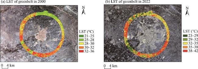
Fig. 3 LST of greenbelt in 2000 (a) and 2022(b)
The second stage is converting radiance to temperature of satellite brightness through applying Equation 2 (Aik et al., 2020):

TB=K2/ln((K1/Lλ)+1),

where TB is the top of atmospheric brightness temperature measured in Kelvin (K); K2 is the band-specific thermal conversion constant 2 (W/(m2•sr•µm)); and K1 is the band-specific thermal conversion constant 1 (W/(m2•sr•µm)).
The third stage involves the computation of normalized difference vegetation index (NDVI) by utilizing the red (Red) and near-infrared (NIR) bands of the Landsat imagery (Sobrino et al., 2004). This is achieved through Equation 3, which can be expressed as follows:

NDVI=(NIR−Red)/(NIR+Red).

The subsequent step involves the computation of the proportion of vegetation (Pv) utilizing Equation 4 (Carlson and Ripley, 1997):

Pv=(NDVI-NDVImin)2/(NDVImax-NDVImin),

where NDVImin is the minimum NDVI; and NDVImax is the maximum NDVI.
The next stage involves the estimation of land surface emissivity (ε) through the application of the model of Valor and Caselles (1996). NDVI-based emissivity method (NBEM) was used in the model, which is employed to determine the emissivity of a certain surface (Sekertekin and Bonafoni, 2020). The emissivity is calculated using Equation 5:

ε=0.985Pv+0.960(1−Pv)+0.06Pv(1−Pv).

The coming step includes calculating LST using Equation 6 (Zhang et al., 2013):

LST=TB/(1+(λ×TB/q) lnε),

where LST is the land surface temperature (K); λ is the wavelength of emitted radiance (µm); and q=h×c/σ (1.438×10⁻² m•K), in which h is the Planck's constant (6.626×10⁻³⁴ J·s); σ is the Boltzmann constant (1.38×10⁻²³ J/K); and c is the velocity of light (2.998×10⁻⁸ m/s).
The final stage is converting LST values from Kelvin to Celsius (Dash et al., 2002):

Tc=LST-273,

where Tc is the LST in Celsius (°C).

3 Results

3.1 LULC and LST

Table 5 displays the variations in the area and mean LST across different LULC classes. In 2000, VL had the highest land area, making up around 56.75% of the overall area. VH comprised 19.94% of the total area, whereas CU and BS accounted for 12.33% and 9.94%, respectively. In contrast, the percentage of the area occupied by BU was the lowest (1.05%). Comparable findings have been identified in 2022.
Table 5 Changes of area and mean LST of different LULC classifications of greenbelt in 2000 and 2022
LULC classification 2000 2022
Area (km2) Percentage (%) Mean LST (°C) Area (km2) Percentage (%) Mean LST (°C)
VL 106.67 56.75 31.63 90.30 48.03 37.64
BU 1.97 1.05 30.42 14.89 7.92 37.65
BS 18.68 9.94 31.64 22.93 12.20 37.65
CU 23.18 12.33 31.76 26.66 14.18 37.87
VH 37.48 19.94 29.48 33.22 17.67 30.34
Concerning LST, in 2020, the lowest LST was 29.48°C in VH, followed by BU (30.42°C), and the highest was found in CU (31.76°C). VL and BS revealed a very slight LST difference. In 2022, the lowest temperature recorded in VH (30.34°C), while the highest temperature recorded in CU (37.87°C). There was no noticeable variation in LST values within the other three landscape types. According to Table 6, LST variance between VH and CU reached 2.28°C in 2000 and 7.53°C in 2022. In addition, LST difference between VH and VL was 2.15°C in 2000 and 7.30°C in 2022, and between VH and BS was 2.16°C in 2000 and 7.31°C in 2022.
Table 6 Difference in LST of greenbelt between VH and the other LULC classifications
LULC
classification
LST of VH
in 2000 (°C)
LST of VH
in 2022 (°C)
LULC
classification
LST of VH
in 2000 (°C)
LST of VH
in 2022 (°C)
VL 2.15 7.30 BS 2.16 7.31
BU 0.94 7.31 CU 2.28 7.53
Variations in LULC area and LST from 2020 to 2022 are illustrated in Figure 4. From 2000 to 2022, VL area witnessed a decline of -8.72%, while LST experienced a notable rise of 6.01°C. However, BU experienced the most substantial expansion in terms of area among the other landscape types, with a growth rate of 6.87%. Concurrently, it was encountered with the greatest increase in LST (7.23°C). Despite a modest rise of 1.85% in CU area, LST exhibited a substantial increase of 6.11°C. The correlation between percentage of LULC area and LST in CU was the greatest (r=0.520; P<0.01). Additionally, BS increased by 2.26%, and LST grew by 6.01°C. A significant positive connection was also observed between percentage of LULC area and LST in BS (r=0.279; P<0.01). VH exhibited a decrease in its size, totaling -2.27%. And it is essential to point out that it was the only one land type in which LST showed a slight increase of 0.83°C. In VH, there was a strong negative relationship between percentage of LULC area and LST (r= -0.482; P<0.01).
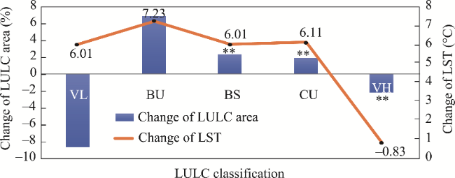
Fig. 4 Changes of LULC area and LST of greenbelt from 2000 to 2022. **, P<0.01 level.

3.2 Landscape metrics of LULC and LST

The differences in land use metrics between 2000 and 2022 by utilizing analysis of variance (t-test) are illustrated in Figure 5. VL and VH, which make up the majority of study area, had similar changing trend of landscape metrics. In parallel with the reduction of total area of both classes, the landscape metrics, namely NP and PD increased significantly from 2000 to 2022. Likewise, the rise in DIVISION and LSI indices provides more evidence of growing disaggregation within these two classes. Although VL had the highest value of LPI among all the land uses in 2000, it witnessed a significant drop in 2022. Furthermore, LPI of VH also experienced a marginal fall and a notable declining trend for both classes.
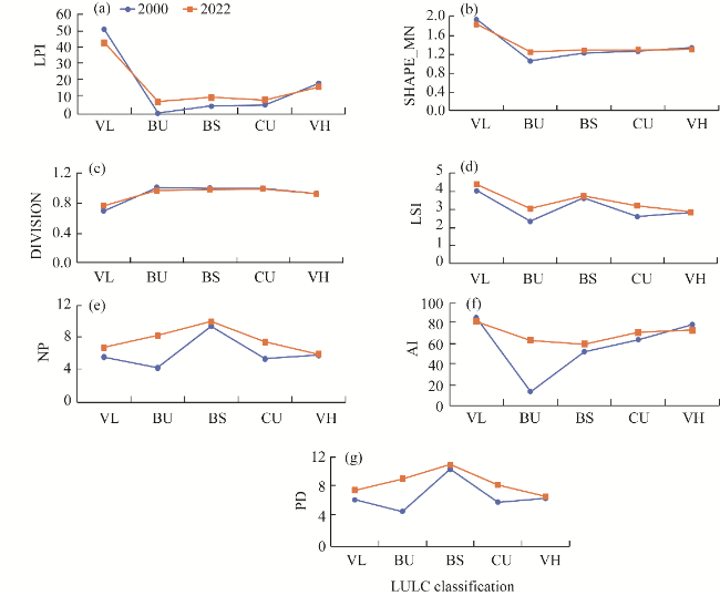
Fig. 5 Variations of landscape metrics of different LULC classifications of greenbelt in 2000 and 2022. (a), LPI; (b), SHAPE_MN; (c), DIVISION; (d), LSI; (e), NP; (f), AI; (g), PD.
Relating to BU, we found an increase in NP in parallel with the growth of its area from 2000 to 2022, which could be noticed in the intensification of total area. Moreover, this result could be revealed by the substantial increase in the value of LPI during the period. Also, the significant rise in SHAPE_MN and LSI indicated that BU was consisting of more irregularly shaped patches. Additionally, there was a considerable increase in AI, supported with the reduction of DIVISION from 2000 to 2022. Although the changes of landscape metrics for CU were not significant, it had a similar trend with BU. There was an observed rise in the values of NP, LPI, and PD, and SHAPE_MN and LSI exhibited an increase, suggesting a shift towards more complex forms rather than simple ones. Conversely, there was a decrease in the values of DIVISION in CU. Regarding BS, the significant growth in the value of LPI can be attributed to the observed rise in the area. Additionally, DIVISION had a decline, providing further evidence that the landscape type became more aggregated. In contrast, both AI and SHAPE_MN exhibited an increase trend throughout the study period.
On the other hand, the Pearson's correlation coefficients indicate that the connection between LST and landscape metrics differed among LULC classifications (Table 7). For VL, the relation between LST and any of the class metrics was not significant. Meanwhile, a strong positive correlation was found between AI and LST in BU; however, none of the other metrics of BU had significant relationship with LST. In BS, LSI, PD, and NP had a strong positive correlation with LST at P<0.01 level; similarly, AI had a positive relation with LST at P<0.05 level. Among other landscape metrics in BS, DIVISION was negatively linked while SHAPE_MN was positively connected, although not significant. The majority of the landscape indices of CU were significant apart from NP and PD. While LPI, AI, LSI, and SHAPE_MN all demonstrated a high significant positive association with LST, DIVISION had a high significant negative relationship with LST at P<0.01 level. The metrics LPI, SHAPE_MN, and AI in VH had a strong significant negative correlation with LST. On the contrary, DIVISION was highly positively correlated with LST and PD had a positive relation with LST at P<0.05 level. Examining the relevance of landscape metrics in relation to LST for LULC classification, the results showed that for VH, the highest value was found in LPI, which in descending order was followed by SHAPE_MN, AI, DIVISION, and PD. For CU, the order was LPI, AI, DIVISION, SHAPE_MN, and LSI. For BS, they were LSI, NP, PD, and AI. The only landscape metric that revealed significant correlation with LST in BU was AI, while VL metrics did not exhibit any significant association with LST during the study period.
Table 7 Pearson's correlation between changes of landscape metrics and LST of greenbelt
Change of landscape metrics in 2000 and 2022 Correlation VL BU BS CU VH
LPI Pearson's correlation -0.028 0.103 0.139 0.451** -0.488**
P 0.750 0.281 0.125 0.000 0.000
n 136 111 123 125 113
SHAPE_MN Pearson's correlation -0.004 0.134 0.163 0.258** -0.475**
P 0.961 0.160 0.071 0.004 0.000
n 136 111 123 125 113
LSI Pearson's correlation 0.014 0.074 0.415** 0.181* 0.023
P 0.868 0.442 0.000 0.044 0.807
n 136 111 123 125 113
DIVISION Pearson's correlation 0.086 -0.086 -0.009 -0.319** 0.374**
P 0.321 0.370 0.919 0.000 0.000
n 136 111 123 125 113
NP Pearson's correlation 0.078 0.069 0.329** 0.106 0.181
P 0.369 0.473 0.000 0.241 0.055
n 136 111 123 125 113
PD Pearson's correlation 0.090 0.064 0.320** 0.111 0.190*
P 0.300 0.504 0.000 0.217 0.043
n 136 111 123 125 113
AI Pearson's correlation -0.158 0.325** 0.199* 0.417** -0.381**
P 0.065 0.001 0.030 0.000 0.000
n 136 95 119 121 109

Note: **, P<0.01 level; *, P<0.05 level.

4 Discussion

4.1 Relationship between LULC classification and LST

The results implied that both the type and percentage of LULC had a relation with LST, which confirmed the importance of landscape composition in minimizing surface temperature within greenbelt in semi-arid areas.
First, the study found that between 2000 and 2022, green spaces, including VH and VL, had declined and been replaced by non-green types comprising BU, BS, and CU. This result can be attributed to the expansion of villages, in addition to the extension of roadways, which thus affects VH within them, including crops and trees. Moreover, the increase of private summer houses due to economic growth since 2003 affected the transition of VL into BU, regardless of whether these farms included a small green area. The result aligns with Rash et al. (2023), who highlighted the encroachment of grasslands by villagers and suburban people, leading to the transformation of green spaces into BU. On one hand, climate change and drought affected the transition of VL into BS (Chavez Rodriguez et al., 2024). On the other hand, the expansion of CU also affected VL. This expansion is due to economic growth and the shift to use mechanical irrigation systems by farmers and landowners. Hamad et al. (2018) have highlighted the effect of economic development on LULC change in the Kurdistan Region of Iraq, examining the effects of human activities—namely agricultural practices—on landscape owing to improved economic circumstances and political stability during the last few decades. Moreover, our results showed variations in the LST of different LULC classifications within these two years. VH was linked to the lowest LST, aligning with the findings of the other studies (Song et al., 2020; Bhagat and Prasad, 2023). Yet, the difference in LST between VH and the other LULC classifications was not high, ranging from 2.00°C to 7.00°C in 2000 and 2022. The reasons might be the fact that VH consisted mostly of crops, vegetables, and shrubs, while limited availability of trees in this classification caused consequences on its cooling effect (Kong et al., 2014). Notably, LST of VL in 2000 and the increase trend in 2022 were similar to those of BS, and differences in LST existed between VH and VL. The results may be explained by the little effect of grass in reducing LST, particularly in the semi-arid areas as grass is more exposed to water stress due to its shallow roots, which might lead it to lose its evapotranspiration function sooner (Myint et al., 2015). This result is consistent with the findings of Yang et al. (2017), who detected that grass had a low cooling effect, while trees had the biggest effects on decreasing LST, compared with shrubs and crops (Bao et al., 2016; Liu et al., 2022b). Thus, in planning greenbelts with semi-arid climate, it is essential to emphasize the types of green space, which mostly comprise trees, followed by shrubs, crops, and vegetables. On the contrary, VL that consists of grass should be less considered by urban and landscape planners.
CU had the highest LST within these two years and the highest LST difference with VH. We observed the same trend for BS but with a slight LST difference with CU. The reasons can be attributed to the characteristics of BS and CU, wherein the absence of vegetation and reduced moisture content eventually cause an increase in the temperature of these surfaces. Rasul et al. (2017) and Azhdari et al. (2018) have confirmed the heating effect of BS in semi-arid areas. However, previous studies have not investigated the heating effect of CU in semi-arid areas.
LST was lower in BU than in BS and CU, and even lower than in VL in 2000. This result can be explained by two reasons: first, most of the village's building material was mud in 2000, which has a low surface temperature (Madhumathi et al., 2014); second, green spaces—including trees and shrubs—occurred in BU, which played an important role in cooling the temperature of BU. However, the trend in 2022 was different in BU as LST was high. The reasons could be related to the change of building material to concrete in 2022, which had a critical impact on elevating LST (Connors et al., 2013). Materials such as cement and tiles, which are commonly used in the construction of buildings, squares, housing developments, roads, and bridges, have been found to release considerable amounts of heat, thus causing elevated temperature (Wang et al., 2017). The results revealed that the temperature of BU in semi-arid areas was mostly correlated with that of urban areas, and LST in BU was lower than that in BS (Rasul et al., 2015).
Additionally, not only the type of landscape but also the changes of LULC classification affect LST. The results of Pearson's correlation revealed variations in the impact of the changes of LULC classification on LST. VH had a significantly negative effect, while VL had no effect. The obtained result is in parallel with the finding from Naeem et al. (2018), who found that increasing the proportion of green space with trees or reducing the percentage of impermeable surfaces can enhance the cooling impact more efficiently. Our findings revealed that CU and BS had significantly positive effects, while BU had no effect. Similar results were also found in other studies (Lai et al., 2012; Li et al., 2013a; Myint et al., 2015; Naeem et al., 2018; Amani-Beni et al., 2019).

4.2 Relationship between landscape metrics and LST

In this study, LULC classification exhibited changes in relation to landscape spatial distribution that had a substantial impact on LST from 2000 to 2022. Specifically, VH patches became more fragmented, heterogeneous, and dispersed owing to increases in NP, LSI, DIVISION, and PD. Nevertheless, only DIVISION and PD had a significantly positive relation. The metrics of LPI, SHAPE_MN, and AI exhibited a reduction in value, resulting in smaller, fragmented, and disaggregated patches. These metrics showed a significantly negative connection with LST. Consequently, the spatial configuration metrics of VH had an impact on LST. However, VL had the same spatial characteristics as VH, but the correlation of VL metrics with LST was not significant; thus, the spatial configuration of VL had no effect on LST. These findings align with that of Hou and Estoque (2020), who found negative correlations of LPI, SHAPE_MN, and AI with LST for VH, while VL metrics had no significant relation. Previous studies conducted by Maimaitiyiming et al. (2014) and Masoudi and Tan (2019) verified the same results. Nevertheless, we observed increases in LPI, NP, SHAPE_MN, LSI, and AI of BU, which suggests a transition to more dominant, aggregated, complex, and irregular patches, whereas the reduction of DIVISION showed aggregation and homogeneity. However, only AI had a substantially positive correlation with LST. The study by Li et al. (2011) demonstrated similar findings, affirming the effect of BU on elevating LST. Our results showed that CU patches became more homogenous, irregular, aggregated, and larger as AI, LPI, SHAPE_MN, and LSI increased. Furthermore, we observed a reduction in DIVISION as indicative of defragmentation with significantly negative association. Madanian et al. (2018) found similar results related to the effects of AI and LPI of harvested agriculture land on rising LST. Our findings revealed that BS became more irregular and complex with increases in SHAPE_MN and LSI in 2022. Additionally, the patches were more contiguous owing to the rise of AI, with a significantly positive correlation. A study by Li et al. (2020) who observed that the scattered arrangement and limited connectivity of BS contributed to the efficient mitigation of warming effects.
The aforementioned results led to the conclusion that VH metrics had the greatest impact, with the highest number of metrics significantly correlated with LST, as similarly recognized in previous studies (Li et al., 2011; Liu et al., 2022b). Conversely, VL metrics had no effect on LST. Consistent with the findings of Azhdari et al. (2018), our study found that CU and BS metrics had high influence on increasing LST. Our findings showed that BU metric did not have a consequential effect on LST. The results are comparable to that of research conducted by Zheng et al. (2014); nevertheless, they differ from other previous researches (Liu and Weng, 2008; Effati et al., 2021), suggesting that BU metrics were effective in rising LST. Our results proved that AI metrics were the most impactful due to their significant correlations with LST in all LULC classifications except VL. The results are similar to those of prior studies by Li et al. (2012) and Estoque et al. (2017), revealing that the defragmentation and aggregation of green and impervious patches had the most consistently significant relation with LST.
Ultimately, we observed variations in the spatial characteristics of LULC and their relation with LST. As VH patches became disaggregated, fragmented, smaller, and regularly consistently shaped, LST increased. In contrast, the elevated surface temperatures of BS and CU were associated with contiguous, aggregated, defragmented, larger, and complex patches. LST in BU increased as the patches layout became more concentrated and aggregated; thus, landscape designers and planners have the responsibility to consider the spatial configuration of LULC by enhancing the cooling impact of VH and reducing the warming effects of CU, BS, and BU within greenbelt in semi-arid areas.

4.3 Implications and limitations

Our findings provide guidelines for concerning urban planning and landscape design. On one hand, it is essential to increase VH by focusing on the availability of denser trees by means of afforestation to decrease BS and VL. Additionally, CU should be converted into agriculture lands by utilizing specific types of vegetation that can grow within greenbelt in all seasons. This approach could reduce the effect of dry CU on elevating LST. On the other hand, urban planners and policymakers should consider optimizing the spatial pattern of specific LULC to mitigate LST; this can be achieved by connecting small patches of VH to produce larger aggregated areas acting as green corridors and by planning irregularly shaped VH within CU and BS to divide the latter into smaller fragmented patches. Similarly, gardens and green spaces with dense trees should be included in villages and main roads to scatter BU layout. Overall, the study provides valuable insights and expands the limited knowledge on the effect of landscape composition and configuration on LST within greenbelt in semi-arid areas to further promote sustainable development.
As the study was concerned with spatial and temporal changes of landscape metrics within a period of two years, it is imperative to have some limitations in the study. Freely remote sensing data with enhanced spatial resolution had accessibility constraints for the whole study period, which affected our ability to obtain precise quantitative outcomes. Furthermore, the limitation of data influenced the classification of LULC without considering their characteristics. For instance, restrictions prevented the consideration of tree species found within VH, as well as the evaluation of greenness, leaf pigments, chlorophyll levels, and water content of vegetation. Additionally, BU had data constraints concerning village block types and building features for the same reason. Moreover, the study depended solely on remotely sensed data of spring daytime to achieve its aims. More researches could be conducted by considering seasonal and nighttime data for analyzing the relationship of landscape pattern with LST. It is important to note that the study had been conducted in Erbil City, Iraq, with a semi-arid climate, and the findings may not be generalized to dissimilar climate areas. Hence, further research employing remote sensing data of higher resolution regarding the detailed parameters of LULC classification is recommended. Further studies might expand upon the present understanding of the relation between spatiotemporal changes of landscape pattern with LST within the greenbelt of other cities with semi-arid climate.

5 Conclusions

The study examined the spatial and temporal changes of LULC and their relations with LST from 2000 to 2022 within an inner greenbelt in the Erbil, a semi-arid city of northern Iraq. From the results, LST may be alleviated by specific types of LULC throughout the planning process. It is recommended to raise VH and attain further improvement by adding a greater number of dense trees. This approach aligns with previous strategies that have emphasized the importance of expanding green spaces in greenbelts. We found that within LULC, it would be beneficial to reduce BS and CU areas. However, in semi-arid areas, raising VL or lowering BU does not make a substantial contribution to attaining a bigger reduction in surface temperature. The most efficient landscape type in providing a cooling effect among all types of LULC classification was VH, which consisted of crops, grains, shrubs, and dispersed trees. Hence, it is crucial for urban planners to prioritize optimizing the spatial configuration of effective LULC to reduce LST within greenbelt in semi-arid areas. It is recommended for VH patches to be larger, aggregated, and concentrated and have a complex shape. However, in addition to scattered BU patches, small, fragmented, dispersed, and regular-shaped patches for BS and CU can contribute to reduce LST. Therefore, LST in greenbelt of semi-arid areas can be altered not only by landscape composition but also by the improvement of its spatial configuration.

Conflict of interest

The authors declare that they have no known competing financial interests or personal relationships that could have appeared to influence the work reported in this paper.

Acknowledgements

The authors are grateful to the editors and anonymous reviewers for their insightful comments.

Author contributions

Conceptualization: Hamid MALIKI, Suzan ISMAIL; Methodology: Hamid MALIKI, Suzan ISMAIL; Formal analysis: Suzan ISMAIL; Writing - original draft preparation: Suzan ISMAIL; Writing - review and editing Hamid MALIKI, Suzan ISMAIL; Funding acquisition: Suzan ISMAIL; Resources: Suzan ISMAIL; Supervision: Hamid MALIKI; Software: Suzan ISMAIL; Visualization: Suzan ISMAIL; Project administration: Hamid MALIKI, Suzan ISMAIL; Data curation: Suzan ISMAIL; Investigation: Suzan ISMAIL; Validation: Suzan ISMAIL. All authors approved the manuscript.
Open Access This article is licensed under a Creative Commons Attribution 4.0 International License, which permits use, sharing, adaptation, distribution and reproduction in any medium or format, as long as you give appropriate credit to the original author(s) and the source, provide a link to the Creative Commons licence, and indicate if changes were made. The images or other third party material in this article are included in the article's Creative Commons licence, unless indicated otherwise in a credit line to the material. If material is not included in the article's Creative Commons licence and your intended use is not permitted by statutory regulation or exceeds the permitted use, you will need to obtain permission directly from the copyright holder. To view a copy of this licence, visit http://creativecommons.org/licenses/by/4.0/.
[1]
Abdullah S A, Nakagoshi N. 2006. Changes in landscape spatial pattern in the highly developing state of Selangor, peninsular Malaysia. Landscape and Urban Planning, 77(3): 263-275.

[2]
Abebe G, Getachew D, Ewunetu A. 2022. Analysing land use/land cover changes and its dynamics using remote sensing and GIS in Gubalafito district, Northeastern Ethiopia. Discover Applied Sciences, 4: 30, doi: 10.1007/S42452-021-04915-8.

[3]
Aik D H J, Ismail M H, Muharam F M. 2020. Land use/land cover changes and the relationship with land surface temperature using Landsat and Modis imageries in Cameron Highlands, Malaysia. Land, 9(10): 372, doi: 10.3390/land9100372.

[4]
Ali K, Johnson B A. 2022. Land-use and land-cover classification in semi-arid areas from medium-resolution remote-sensing imagery: A deep learning approach. Sensors, 22(22): 8750, doi: 10.3390/s22228750.

[5]
Amani-Beni M, Zhang B, Xie G Di, et al. 2019. Impacts of urban green landscape patterns on land surface temperature: Evidence from the adjacent area of Olympic Forest Park of Beijing, China. Sustainability, 11(2): 513, doi: 10.3390/su11020513.

[6]
Amati M. 2016. Urban Green Belts in the Twenty-first Century. Oxford: Routledge, 268.

[7]
Anderson J R, Hardy E E, Roach J T, et al. 1976. A land use and land cover classification system for use with remote sensor data. [2023-12-09]. https://pubs.usgs.gov/publication/pp964.

[8]
Athukorala D, Murayama Y. 2020. Spatial variation of land use/cover composition and impact on surface urban heat island in a tropical sub-Saharan city of Accra, Ghana. Sustainability, 12(19): 7953, doi: 10.3390/SU12197953.

[9]
Azhdari A, Soltani A, Alidadi M. 2018. Urban morphology and landscape structure effect on land surface temperature: Evidence from Shiraz, a semi-arid city. Sustainable Cities and Society, 41: 853-864.

[10]
Balany F, Ng A W, Muttil N, et al. 2020. Green infrastructure as an urban heat island mitigation strategy-a review. Water, 12(12): 3577, doi: 10.3390/w12123577.

[11]
Bao T, Li X M, Zhang J, et al. 2016. Assessing the distribution of urban green spaces and its anisotropic cooling distance on urban heat island pattern in Baotou, China. ISPRS International Journal of Geo-Information, 5(2): 12, doi: 10.3390/ijgi5020012.

[12]
Baper S, Hassan A, Ismail S. 2013. Modernization theory and house garden transformation: Erbil City as case study. Scientific Journal of Koya University, 1(1): 7-13.

[13]
Bengston D N, Youn Y C. 2006. Urban containment policies and the protection of natural areas: The case of Seoul's greenbelt. Ecology and Society, 11(1): 3, doi: 10.5751/ES-01504-110103.

[14]
Bhagat S, Prasad P R C. 2023. Assessing the impact of spatio-temporal land use and land cover changes on land surface temperature, with a major emphasis on mining activities in the state of Chhattisgarh, India. Spatial Information Research, 32: 339-355.

[15]
Carlson T N, Ripley D A. 1997. On the relation between NDVI, fractional vegetation cover, and leaf area index. Remote Sensing of Environment, 62(3): 241-252.

[16]
Chavez Rodriguez L, Parker S, Fiore N M, et al. 2024. Impact of drought on ecohydrology of southern California grassland and shrubland. Ecosystems, 27(1): 106-121.

[17]
Connors J P, Galletti C S, Chow W T L. 2013. Landscape configuration and urban heat island effects: Assessing the relationship between landscape characteristics and land surface temperature in Phoenix, Arizona. Landscape Ecology, 28(2): 271-283.

[18]
Dash P, Göttsche F M, Olesen F S, et al. 2002. Land surface temperature and emissivity estimation from passive sensor data: Theory and practice-current trends. International Journal of Remote Sensing, 23(13): 2563-2594.

[19]
Debie E, Anteneh M, Asmare T. 2022. Land use/cover changes and surface temperature dynamics over Abaminus watershed, Northwest Ethiopia. Air, Soil and Water Research, 15: 11786221221097917, doi: 10.1177/11786221221097917.

[20]
Effati F, Karimi H, Yavari A. 2021. Investigating effects of land use and land cover patterns on land surface temperature using landscape metrics in the city of Tehran, Iran. Arabian Journal of Geosciences, 14(13): 1240, doi: 10.1007/s12517-021-07433-4.

[21]
Estoque R C, Murayama Y, Myint S W. 2017. Effects of landscape composition and pattern on land surface temperature: An urban heat island study in the megacities of Southeast Asia. Science of the Total Environment, 577: 349-359.

[22]
Fan C, Myint S. 2014. A comparison of spatial autocorrelation indices and landscape metrics in measuring urban landscape fragmentation. Landscape and Urban Planning, 121: 117-128.

[23]
Galvez R A, Louis F, Dagoc S, et al. 2024. Modeling the influence of land cover dynamics on spatio-temporal variations in land surface temperature in Cagayan de Oro River basin, Mindanao, Philippines. Modeling Earth Systems and Environment, 10(1): 899-912.

[24]
Gaznayee H A A, Al-Quraishi A M F, Mahdi K, et al. 2022. A geospatial approach for analysis of drought impacts on vegetation cover and land surface temperature in the Kurdistan Region of Iraq. Water, 14(6): 927, doi: 10.3390/w14060927,

[25]
Hamad R, Kolo K, Land H B. 2018. Post-war land cover changes and fragmentation in Halgurd Sakran National Park (HSNP), Kurdistan region of Iraq. Land, 7(1): 38, doi: 10.3390/land7010038.

[26]
Han A T, Daniels T L, Kim C. 2022. Managing urban growth in the wake of climate change: Revisiting greenbelt policy in the US. Land Use Policy, 112: 105867, doi: 10.1016/j.landusepol.2021.105867.

[27]
Han H Y, Huang C, Ahn K H, et al. 2017. The effects of greenbelt policies on land development: Evidence from the deregulation of the greenbelt in the Seoul metropolitan area. Sustainability, 9(7): 1259, doi: 10.3390/su9071259.

[28]
Hou H, Estoque R C. 2020. Detecting cooling effect of landscape from composition and configuration: An urban heat island study on Hangzhou. Urban Forestry and Urban Greening, 53: 126719, doi: 10.1016/j.ufug.2020.126719.

[29]
Jia X L, Song P H, Yun G L, et al. 2022. Effect of landscape structure on land surface temperature in different essential urban land use Categories: A case study in Jiaozuo, China. Land, 11(10): 1687, doi: 10.3390/land11101687

[30]
Kardani-Yazd N, Kardani-Yazd N, Mansouri Daneshvar M R. 2019. Strategic spatial analysis of urban greenbelt plans in Mashhad city, Iran. Environmental Systems Research, 8: 30, doi: 10.1186/s40068-019-0158-9.

[31]
Kong F H, Yin H W, James P, et al. 2014. Effects of spatial pattern of greenspace on urban cooling in a large metropolitan area of eastern China. Landscape and Urban Planning, 128: 35-47.

[32]
Kumari M, Sarma K. 2017. Changing trends of land surface temperature in relation to land use/cover around thermal power plant in Singrauli district, Madhya Pradesh, India. Spatial Information Research, 25: 769-777.

[33]
Lai Y J, Li C F, Lin P H, et al. 2012. Comparison of MODIS land surface temperature and ground-based observed air temperature in complex topography. International Journal of Remote Sensing, 33(24): 7685-7702.

[34]
Li J X, Song C H, Cao L, et al. 2011. Impacts of landscape structure on surface urban heat islands: A case study of Shanghai, China. Remote Sensing of Environment, 115(12): 3249-3263.

[35]
Li X M, Zhou W Q, Ouyang Z Y. 2013a. Relationship between land surface temperature and spatial pattern of greenspace: What are the effects of spatial resolution? Landscape and Urban Planning, 114: 1-8, doi: 10.1016/j.landurbplan.2013.02.005.

[36]
Li X M, Zhou W Q. 2019. Optimizing urban greenspace spatial pattern to mitigate urban heat island effects: Extending understanding from local to the city scale. Urban Forestry and Urban Greening, 41: 255-263.

[37]
Li Y L, Ren C, Ho J Y E, et al. 2023. Landscape metrics in assessing how the configuration of urban green spaces affects their cooling effect: A systematic review of empirical studies. Landscape and Urban Planning, 239: 104842, doi: 10.1016/j.landurbplan.2023.104842.

[38]
Li Z L, Tang B H, Wu H, et al. 2013b. Satellite-derived land surface temperature: Current status and perspectives. Remote Sensing of Environment, 131: 14-37.

[39]
Liang S L, Wang J D. 2019. Advanced Remote Sensing:Terrestrial Information Extraction and Applications. Pittsburgh: Academic Press.

[40]
Liu H, Weng Q H. 2008. Seasonal variations in the relationship between landscape pattern and land surface temperature in Indianapolis, USA. Environmental Monitoring and Assessment, 144: 199-219.

[41]
Liu S, Li X F, Chen L, et al. 2022a. A new approach to investigate the spatially heterogeneous in the cooling effects of landscape pattern. Land, 11(2): 239, doi: 10.3390/land11020239.

[42]
Liu W R, Jia B Q, Li T, et al. 2022b. Correlation analysis between urban green space and land surface temperature from the perspective of spatial heterogeneity: A case study within the sixth ring road of Beijing. Sustainability, 14(20): 13492, doi: 10.3390/su142013492.

[43]
Madanian M, Soffianian A R, Koupai S S, et al. 2018. Analyzing the effects of urban expansion on land surface temperature patterns by landscape metrics: A case study of Isfahan City, Iran. Environmental Monitoring and Assessment, 189: 190, doi: 10.1007/s10661-018-6564-z.

[44]
Madhumathi A, Vishnupriya J, Vignesh S. 2014. Sustainability of traditional rural mud houses in Tamilnadu, India: An analysis related to thermal comfort. Journal of Multidisciplinary Engineering Science and Technology, 1(5): 302-311.

[45]
Maimaitiyiming M, Ghulam A, Tiyip T, et al. 2014. Effects of green space spatial pattern on land surface temperature: Implications for sustainable urban planning and climate change adaptation. ISPRS Journal of Photogrammetry and Remote Sensing, 89: 59-66.

[46]
Masoudi M, Tan P Y. 2019. Multi-year comparison of the effects of spatial pattern of urban green spaces on urban land surface temperature. Landscape and Urban Planning, 184: 44-58.

[47]
McGarigal K, Marks B J. 1995. Spatial pattern analysis program for quantifying landscape structure. In: General Technical Report. PNW-GTR-351. United States Department of Agriculture, Forest Service, Pacific Northwest Research Station, USA.

[48]
McGarigal K. 2014. Fragstats Help. Amherst: University of Massachusetts: 182.

[49]
McGarigal K, Cushman S A, Ene E. 2023. Fragstats v.4.0. [2024-01-12]. https://fragstats.org/index.php/downloads.

[50]
Moravec D, Komárek J, Medina S L C, et al. 2021. Effect of atmospheric corrections on NDVI: Intercomparability of Landsat 8, Sentinel-2, and UAV sensors. Remote Sensing, 13(18): 3550, doi: 10.3390/rs13183550.

[51]
Myint S W, Zheng B J, Talen E, et al. 2015. Does the spatial arrangement of urban landscape matter? Examples of urban warming and cooling in phoenix and Las Vegas. Ecosystem Health and Sustainability, 1(4): 1-15.

[52]
Naeem S, Cao C X, Qazi W A, et al. 2018. Studying the association between green space characteristics and land surface temperature for sustainable urban environments: An analysis of Beijing and Islamabad. ISPRS International Journal of Geo-Information, 7(2): 38, doi: 10.3390/ijgi7020038.

[53]
O'Neill R V, Krummel J R, Gardner R H, et al. 1988. Indices of landscape pattern. Landscape Ecology, 1: 153-162.

[54]
Quattrochi D A, Luvall J C. 2014. Thermal infrared remote sensing for analysis of landscape ecological processes: Current insights and trends. Scale Issues in Remote Sensing, 14: 34-60.

[55]
Rash A, Mustafa Y, Hamad R. 2023. Quantitative assessment of Land use/land cover changes in a developing region using machine learning algorithms: A case study in the Kurdistan Region, Iraq. Heliyon, 9(11): e21253, doi: 10.1016/j.heliyon.2023.e21253.

[56]
Rasul A, Balzter H, Smith C. 2015. Spatial variation of the daytime Surface Urban Cool Island during the dry season in Erbil, Iraqi Kurdistan, from Landsat 8. Urban Climate, 14: 176-186.

[57]
Rasul A, Balzter H, Smith C. 2017. Applying a normalized ratio scale technique to assess influences of urban expansion on land surface temperature of the semi-arid city of Erbil. International Journal of Remote Sensing, 38(13): 3960-3980.

[58]
Rimal B, Sharma R, Kunwar R, et al. 2019. Effects of land use and land cover change on ecosystem services in the Koshi River Basin, Eastern Nepal. Ecosystem Services, 38: 100963, doi: 10.1016/j.ecoser.2019.100963.

[59]
Sekertekin A, Bonafoni S. 2020. Land surface temperature retrieval from Landsat 5, 7, and 8 over rural areas: Assessment of different retrieval algorithms and emissivity models and toolbox implementation. Remote Sensing, 12(2): 294, doi: 10.3390/rs12020294.

[60]
Senanayake I P, Welivitiya W D D P, Nadeeka P M. 2013. Remote sensing based analysis of urban heat islands with vegetation cover in Colombo city, Sri Lanka using Landsat-7 ETM+ data. Urban Climate, 5: 19-35.

[61]
Sobrino J A, Jiménez-Muñoz J C, Paolini L. 2004. Land surface temperature retrieval from Landsat TM 5. Remote Sensing of Environment, 90(4): 434-440.

[62]
Song Y, Song X D, Shao G F. 2020. Effects of green space patterns on urban thermal environment at multiple spatial-temporal scales. Sustainability, 12(17): 6850, doi: 10.3390/SU12176850.

[63]
Turner M G. 2005. Landscape ecology: What is the state of the science? Annual Review of Ecology, Evolution, and Systematics, 36: 319-344.

[64]
Valor E, Caselles V. 1996. Mapping land surface emissivity from NDVI: Application to European, African, and South American areas. Remote Sensing of Environment, 57(3): 167-184.

[65]
Vanderhaegen S, Canters F. 2010. Developing urban metrics to describe the morphology of urban areas at block level. International Archives of the Photogrammetry, Remote Sensing and Spatial Information Sciences, 36: 192-197.

[66]
Wang H B, Li H, Ming H B, et al. 2014. Past land use decisions and socioeconomic factors influence urban greenbelt development: A case study of Shanghai, China. Landscape Ecology, 29: 1759-1770.

[67]
Wang H T, Zhang Y Z, Tsou J Y, et al. 2017. Surface urban heat island analysis of Shanghai (China) based on the change of land use and land cover. Sustainability, 9(9): 1538, doi: 10.3390/su9091538.

[68]
Wang Q, Xiong K N, Zhou J Y, et al. 2023. Impact of land use and land cover change on the landscape pattern and service value of the village ecosystem in the karst desertification control. Frontiers in Environmental Science, 11: 1020331, doi: 10.3389/fenvs.2023.1020331.

[69]
Yang C B, He X Y, Yu L X, et al. 2017. The cooling effect of urban parks and its monthly variations in a snow climate city. Remote Sensing, 9(10): 1066, doi: 10.3390/rs9101066.

[70]
Yang J, Jin X. 2007. The failure and success of greenbelt program in Beijing. Urban Forestry and Urban Greening, 6(4): 287-296.

[71]
Zhang H, Qi Z F, Ye X Y, et al. 2013. Analysis of land use/land cover change, population shift, and their effects on spatiotemporal patterns of urban heat islands in metropolitan Shanghai, China. Applied Geography, 44: 121-133.

[72]
Zheng B J, Myint S W, Fan C. 2014. Spatial configuration of anthropogenic land cover impacts on urban warming. Landscape and Urban Planning, 130: 104-111.

[73]
Zhou W Q, Wang J, Cadenasso M L. 2017. Effects of the spatial configuration of trees on urban heat mitigation: A comparative study. Remote Sensing of Environment, 195: 1-12.

文章导航

/