
Construction and optimization of ecological security pattern in the mainstream of the Tarim River Basin, China
Received date: 2024-10-26
Revised date: 2025-04-09
Accepted date: 2025-04-25
Online published: 2025-08-13
QIN Xiaolin , LIU Wei , LING Hongbo , ZHANG Guangpeng , GONG Yanming , MENG Xiangdong , SHAN Qianjuan . [J]. Journal of Arid Land, 2025 , 17(6) : 735 -753 . DOI: 10.1007/s40333-025-0102-y
Scientifically constructing an ecological security pattern (ESP) is an important spatial analysis approach to improve ecological functions in arid areas and achieve sustainable development. However, previous research methods ignored the complex trade-offs between ecosystem services in the process of constructing ESP. Taking the mainstream of the Tarim River Basin (MTRB), China as the study area, this study set seven risk scenarios by applying Ordered Weighted Averaging (OWA) model to trade-off the importance of the four ecosystem services adopted by this study (water conservation, carbon storage, habitat quality, and biodiversity conservation), thereby identifying priority protection areas for ecosystem services. And then, this study identified ecological sources by integrating ecosystem service importance with eco-environmental sensitivity. Using circuit theory, the ecological corridors and nodes were extracted to construct the ESP. The results revealed significant spatial heterogeneity in the four ecosystem services across the study area, primarily driven by hydrological gradients and human activity intensity. The ESP of the MTRB included 34 ecological sources with a total area of 1471.38 km², 66 ecological corridors with a length of about 1597.45 km, 11 ecological pinch points, and 13 ecological barrier points distributed on the ecological corridors. The spatial differentiation of the ESP was obvious, with the upper and middle reaches of the MTRB having a large number of ecological sources and exhibiting higher clustering of ecological corridors compared with the lower reaches. The upper and middle reaches require ecological protection to sustain the existing ecosystem, while the lower reaches need to carry out ecological restoration measures including desertification control. Overall, this study makes up for the shortcomings of constructing ESP simply by spatial superposition of ecosystem service functions and can effectively improve the robustness and stability of ESP construction.
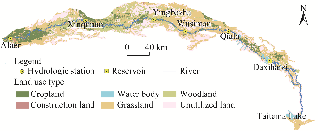
Fig. 1 Overview the spatial distribution of land use in the mainstream of the Tarim River Basin (MTRB) in 2020. The image is from the Resource and Environmental Science Data Center, Chinese Academy of Sciences (https://www.resdc.cn/). |
Table 1 Detailed description of data used in the study |
| Data item | Data source | Resolution |
|---|---|---|
| Land cover | GlobeLand 30 (https://www.globeland30.org/) | 30 m |
| Digital elevation model (DEM) | Geospatial Data Cloud (https://www.gscloud.cn) | 30 m |
| Slope | Geospatial Data Cloud (https://www.gscloud.cn) | 30 m |
| Temperature | MOD11A2 product (https://ladsweb.modaps.eosdis.nasa.gov) | 1 km |
| Precipitation | Global Resource Data Cloud (www.gis5g.com) | 1 km |
| Surface reflectance | MOD09A1 product (https://ladsweb.modaps.eosdis.nasa.gov/) | 500 m |
| Net primary production (NPP) | EARTHDATA (https://ladsweb.modaps.eosdis.nasa.gov/) | 500 m |
| Distance to road (primary road, secondary road, and railway) | Open Street Map (http://www.openstreetmap.org/) | 500 m |
| Distance to water body | Open Street Map (http://www.openstreetmap.org/) | 500 m |
| Groundwater depth | The Tarim River Basin Management Bureau | 500 m |
| River network density | Open Street Map (http://www.openstreetmap.org/) | 500 m |
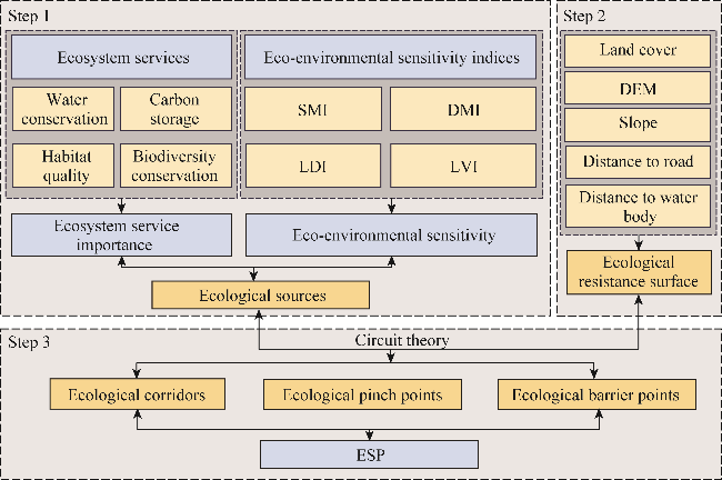
Fig. 2 Construction and optimization framework of ecological security pattern (ESP). DEM, digital elevation model; SMI, salinization monitoring index; DMI, desertification monitoring index; LVI, landscape vulnerability index; LDI, landscape disturbance index. |
Table 2 Carbon density of different land use types in the mainstream of the Tarim River Basin (MTRB) |
| Land use type | Cabove (t C/hm2) | Cbelow (t C/hm2) | Csoil (t C/hm2) | Cdead (t C/hm2) |
|---|---|---|---|---|
| Cropland | 3.47 | 4.12 | 86.22 | 1.24 |
| Woodland | 36.97 | 10.91 | 121.35 | 2.48 |
| Grassland | 0.58 | 5.13 | 85.02 | 0.22 |
| Water body | 0.76 | 0.54 | 0.00 | 0.00 |
| Construction land | 1.88 | 1.74 | 0.00 | 0.00 |
| Unutilized land | 0.54 | 1.04 | 43.39 | 0.00 |
Table 3 Resistance value of each ecological resistance factor involved in this study |
| Resistance factor | Resistance value | Weight | ||||
|---|---|---|---|---|---|---|
| 1.00 | 2.00 | 3.00 | 4.00 | 5.00 | ||
| Land cover | Woodland and water body | Grassland | Cropland | Unutilized land | Construction land | 0.3415 |
| DEM (m) | 765-795 | 795-825 | 825-885 | 885-975 | >975 | 0.0660 |
| Slope (°) | 0-5 | 5-15 | 15-25 | 25-35 | 35-53 | 0.2168 |
| Distance to road (primary road, secondary, and railway) (m) | >700 | 400-700 | 300-400 | 100-300 | <100 | 0.2823 |
| Distance to water body (m) | <100 | 100-300 | 300-500 | 500-1000 | >1000 | 0.0934 |
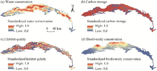
Fig. 3 Spatial distribution of ecosystem service in the MTRB in 2020. (a), water conservation; (b), carbon storage; (c), habitat quality; (d), biodiversity conservation. |
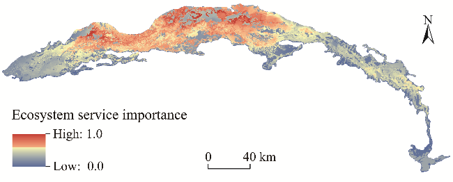
Fig. 4 Spatial distribution of ecosystem service importance in the MTRB in 2020 |
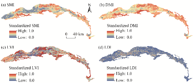
Fig. 5 Spatial distribution of SMI (a), DMI (b), LVI (c), and LDI (d) in the MTRB in 2020 |
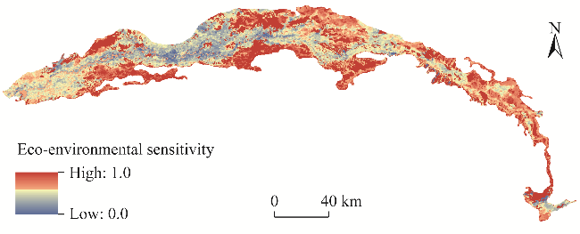
Fig. 6 Spatial distribution of eco-environmental sensitivity in the MTRB in 2020 |
Table 4 Ecological risk and trade-offs between ecosystem services under different scenarios |
| Scenario | Ecological risk | Weight | Ecological trade-off | |||
|---|---|---|---|---|---|---|
| Water conservation | Carbon storage | Habitat quality | Biodiversity conservation | |||
| 1 | 0.0001 | 0.0000 | 0.0000 | 0.0000 | 1.0000 | 0.0000 |
| 2 | 0.1000 | 0.0000 | 0.0550 | 0.0010 | 0.9440 | 0.0740 |
| 3 | 0.5000 | 0.0620 | 0.3120 | 0.1880 | 0.4380 | 0.6770 |
| 4 | 1.0000 | 0.2500 | 0.2500 | 0.2500 | 0.2500 | 1.0000 |
| 5 | 2.0000 | 0.5000 | 0.1590 | 0.2070 | 0.1340 | 0.6610 |
| 6 | 10.0000 | 0.8710 | 0.0390 | 0.0620 | 0.0280 | 0.1720 |
| 7 | 10,000.0000 | 1.0000 | 0.0000 | 0.0000 | 0.0000 | 0.0000 |
Table 5 Ecosystem service conservation efficiency under different scenarios |
| Scenario | Ecological risk | Weight | Conservation efficiency | |||
|---|---|---|---|---|---|---|
| Water conservation | Carbon storage | Habitat quality | Biodiversity conservation | |||
| 1 | 0.0001 | 1.2070 | 1.2310 | 1.4890 | 1.2720 | 1.3000 |
| 2 | 0.1000 | 1.2320 | 1.2560 | 1.5120 | 1.2980 | 1.3250 |
| 3 | 0.5000 | 1.3010 | 1.5530 | 1.7780 | 1.4220 | 1.5140 |
| 4 | 1.0000 | 1.4490 | 1.6500 | 1.8160 | 1.8770 | 1.6980 |
| 5 | 2.0000 | 1.5460 | 1.6670 | 1.8210 | 2.2830 | 1.8290 |
| 6 | 10.0000 | 1.5350 | 1.6610 | 1.8060 | 2.5510 | 1.8880 |
| 7 | 10,000.0000 | 1.5370 | 1.6540 | 1.8020 | 2.5850 | 1.8950 |
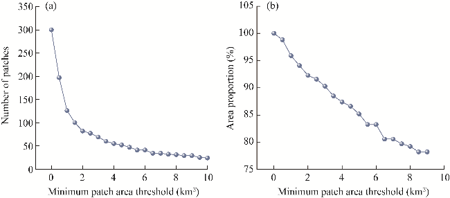
Fig. 7 Effect of the minimum patch area threshold on the number (a) and area proportion (b) of patches |
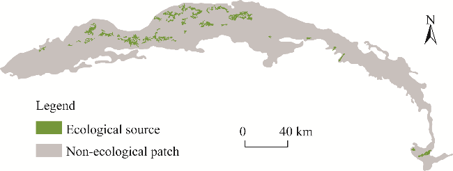
Fig. 8 Spatial distribution of ecological sources in the MTRB in 2020 |
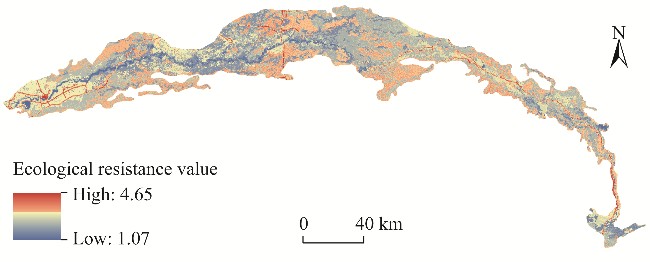
Fig. 9 Spatial distribution of ecological resistance surface in the MTRB in 2020 |
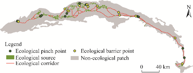
Fig. 10 Distribution of ESP in the MTRB |
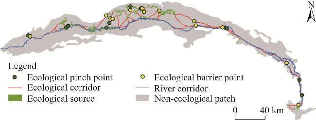
Fig. 11 Optimized layout of ecological corridors with river corridors in the MTRB in 2020 |
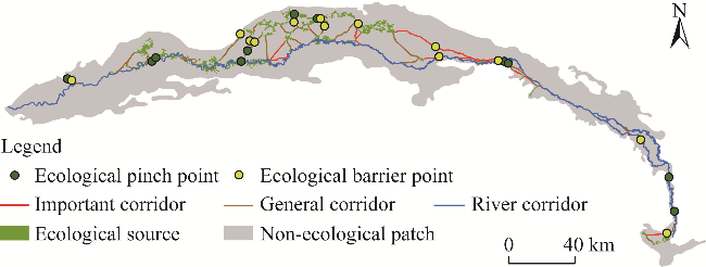
Fig. 12 Distribution of the ESP with the importance of ecological corridors in the MTRB in 2020 |
| [1] |
|
| [2] |
|
| [3] |
|
| [4] |
|
| [5] |
|
| [6] |
|
| [7] |
|
| [8] |
|
| [9] |
|
| [10] |
|
| [11] |
|
| [12] |
|
| [13] |
|
| [14] |
|
| [15] |
|
| [16] |
|
| [17] |
|
| [18] |
|
| [19] |
|
| [20] |
|
| [21] |
|
| [22] |
|
| [23] |
|
| [24] |
|
| [25] |
|
| [26] |
|
| [27] |
|
| [28] |
|
| [29] |
|
| [30] |
|
| [31] |
|
| [32] |
|
| [33] |
|
| [34] |
|
| [35] |
|
| [36] |
|
| [37] |
|
| [38] |
|
| [39] |
|
| [40] |
|
| [41] |
|
| [42] |
|
| [43] |
|
| [44] |
|
| [45] |
|
| [46] |
|
| [47] |
|
| [48] |
|
| [49] |
|
| [50] |
|
| [51] |
|
| [52] |
|
| [53] |
|
| [54] |
|
| [55] |
|
| [56] |
|
| [57] |
|
| [58] |
|
| [59] |
|
| [60] |
|
| [61] |
|
| [62] |
|
| [63] |
|
| [64] |
|
| [65] |
|
| [66] |
|
/
| 〈 |
|
〉 |