• LU Rui 1, 2 ,
  • ZHANG Mingjun , 1, 2, * ,
  • ZHANG Yu 1, 2 ,
  • QIANG Yuquan 1, 2 ,
  • CHE Cunwei 1, 2 ,
  • SUN Meiling 1, 2 ,
  • WANG Shengjie 1, 2
展开

收稿日期: 2024-07-13

  修回日期: 2024-10-30

  录用日期: 2024-11-02

  网络出版日期: 2025-08-13

Estimation of evapotranspiration from artificial forest in mountainous areas of western Loess Plateau based on HYDRUS-1D model

  • LU Rui 1, 2 ,
  • ZHANG Mingjun , 1, 2, * ,
  • ZHANG Yu 1, 2 ,
  • QIANG Yuquan 1, 2 ,
  • CHE Cunwei 1, 2 ,
  • SUN Meiling 1, 2 ,
  • WANG Shengjie 1, 2
Expand
  • 1College of Geography and Environmental Science, Northwest Normal University, Lanzhou 730070, China
  • 2Key Laboratory of Resource Environment and Sustainable Development of Oasis, Gansu Province, Lanzhou 730070, China
*ZHANG Mingjun ()

Received date: 2024-07-13

  Revised date: 2024-10-30

  Accepted date: 2024-11-02

  Online published: 2025-08-13

本文引用格式

LU Rui , ZHANG Mingjun , ZHANG Yu , QIANG Yuquan , CHE Cunwei , SUN Meiling , WANG Shengjie . [J]. Journal of Arid Land, 2024 , 16(12) : 1664 -1685 . DOI: 10.1007/s40333-024-0112-1

Abstract

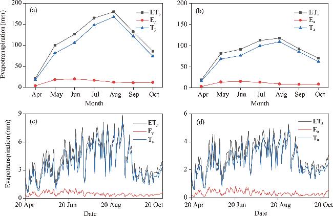
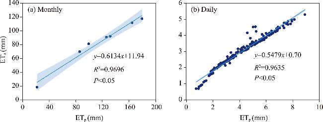
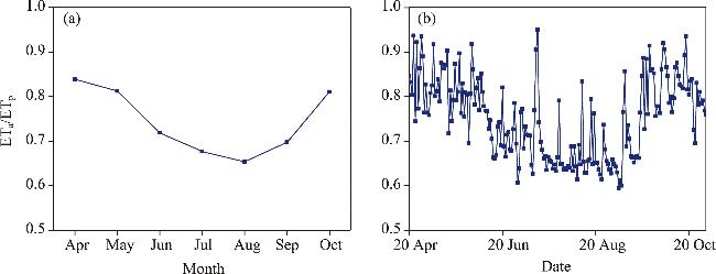
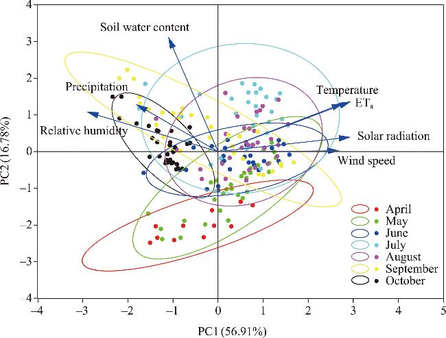
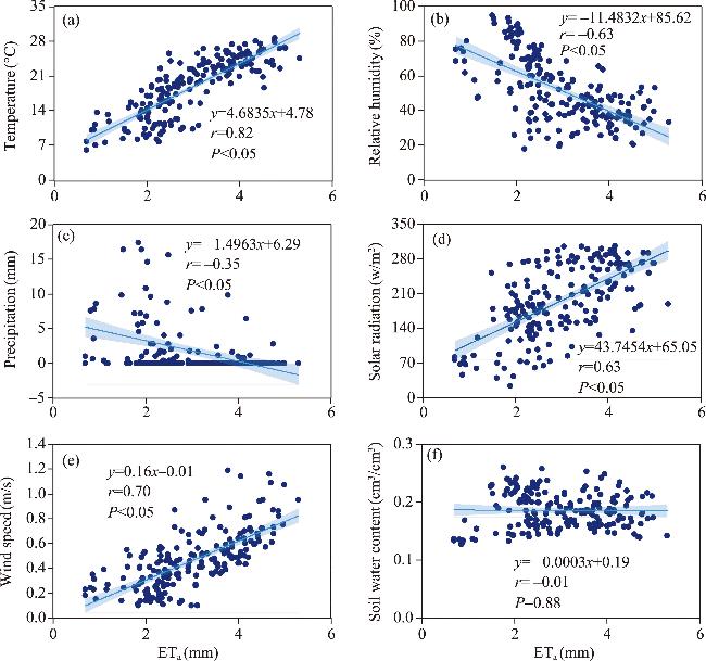
Evapotranspiration is the most important expenditure item in the water balance of terrestrial ecosystems, and accurate evapotranspiration modeling is of great significance for hydrological, ecological, agricultural, and water resource management. Artificial forests are an important means of vegetation restoration in the western Loess Plateau, and accurate estimates of their evapotranspiration are essential to the management and development of water use strategies for artificial forests. This study estimated the soil moisture and evapotranspiration based on the HYDRUS-1D model for the artificial Platycladus orientalis (L.) Franco forest in western mountains of Loess Plateau, China from 20 April to 31 October, 2023. Moreover, the influence factors were identified by combining the correlation coefficient method and the principal component analysis (PCA) method. The results showed that HYDRUS-1D model had strong applicability in portraying hydrological processes in this area and revealed soil water surplus from 20 April to 31 October, 2023. The soil water accumulation was 49.64 mm; the potential evapotranspiration (ETp) was 809.67 mm, which was divided into potential evaporation (Ep; 95.07 mm) and potential transpiration (Tp; 714.60 mm); and the actual evapotranspiration (ETa) was 580.27 mm, which was divided into actual evaporation (Ea; 68.27 mm) and actual transpiration (Ta; 512.00 mm). From April to October 2023, the ETp, Ep, Tp, ETa, Ea, and Ta first increased and then decreased on both monthly and daily scales, exhibiting a single-peak type trend. The average ratio of Ta/ETa was 0.88, signifying that evapotranspiration mainly stemmed from transpiration in this area. The ratio of ETa/ETp was 0.72, indicating that this artificial forest suffered from obvious drought stress. The ETp was significantly positively correlated with ETa, and the R2 values on the monthly and daily scales were 0.9696 and 0.9635 (P<0.05), respectively. Furthermore, ETa was significantly positively correlated with temperature, solar radiation, and wind speed, and negatively correlated with relative humidity and precipitation (P<0.05); and temperature exhibited the highest correlation with ETa. Thus, ETp and temperature were the decisive contributors to ETa in this area. The findings provide an effective method for simulating regional evapotranspiration and theoretical reference for water management of artificial forests, and deepen understanding of effects of each influence factors on ETa in arid areas.

1 Introduction

Evapotranspiration is the dominant expenditure item in the water balance of terrestrial ecosystems. About 70.00% of the global surface precipitation returns to the atmosphere through evapotranspiration, and this value is more than 90.00% in arid areas (Wegehenkel et al., 2017). Evapotranspiration includes transpiration from plant and evaporation from soil. Additionally, it is the main pathway for water balance and energy exchange in soil-plant-atmosphere interface and is the link between key ecological processes, such as stomatal behavior of plants, water use, and carbon exchange (Chen et al., 2023). Evaporation and transpiration are critical elements governing the water balance and energy exchange among soil, vegetation, and atmosphere, and they are closely related to the climatic environment (e.g., solar radiation, temperature, and precipitation), vegetation type (e.g., tree, grass, and shrub), and vegetation growth condition (Lü et al., 2024). In good ecosystems, evaporation and transpiration have an appropriate ratio, for example, transpiration may be two to three times higher than evaporation in a forest ecosystem. An accurate understanding of evaporation and transpiration variations is of great practical significance for assessing and managing soil water in terrestrial ecosystems (Wolf et al., 2024).
Evapotranspiration is subdivided into potential evapotranspiration (ETp) and actual evapotranspiration (ETa). The ETp denotes the upper limit of evapotranspiration relative to the atmospheric evapotranspiration when sufficient sources of surface water are present, and it describes the ability of atmosphere to absorb surface water through evaporation and transpiration (Okkan et al., 2024). The ETa is the actual surface evapotranspiration under the interference of external factors. Peng et al. (2017) determined that ETp would continue to increase in the future, while Lü et al. (2019) suggested that ETa decreases with increasing ETp. However, Su et al. (2021) observed that ETp is positively correlated with ETa, which is closely related to environmental differences and anthropogenic disturbances (Yang et al., 2022). The ratio of ETa/ETp is one of the main climate controlling factors for the distribution of vegetation on land or globally and plays an important role in quantifying the response of vegetation to climate. This ratio can be used to assess the effects of drought stress on plant growth (Ramos et al., 2023). The variations of the ratio of ETa/ETp that stem from increasing aridity and global warming could alter soil water and vegetation cover status, thereby affecting water and carbon cycles (Feng et al., 2018). Therefore, the relationship between ETa and ETp needs to be accurately studied to quantify the water deficit in drylands and predict the ecohydrological response to climate change in drylands.
Numerical modeling is an important tool for deconstructing water balance and reproducing water cycle processes (Xiang et al., 2020). It can effectively simulate hydrological processes and evaluate water resources based on a small number of observations, and advantageously, it requires lower cost, time, and effort than other methods (Chen et al., 2021). The conventional approach to soil water research is characterized by a significant workload, high cost, and varying degrees of outside interference. The integration of traditional field observations with numerical simulation aims to improve the model simulation accuracy while enhancing the operational efficiency. Furthermore, this approach enables the investigation of diverse spatiotemporal scales of soil moisture dynamics and hydrological processes (Diongue et al., 2023). Based on Richards principle, HYDRUS-1D model considers soil hydrothermal and the water absorption processes of root (Thayalakumaran et al., 2018) and has good applicability and operability in simulating the soil water transport and the evapotranspiration dynamics of plants (Wu et al., 2023). Owing to flexible input and output functions and parameter optimization module, HYDRUS-1D model has been widely used (Kumar et al., 2023). Numerous studies have presented the applicability of HYDRUS-1D model in quantifying evapotranspiration (Li et al., 2019; Er-Raki et al., 2021; Lu et al., 2024). For example, Beyene et al. (2018) utilized HYDRUS-1D model to numerically simulate deep percolation and ETa from flood irrigation in the in the floodplains of Lake Tana, Ethiopia, showing HYDRUS-1D model can be used as an effective method to predict deep infiltration and ETa. Lian et al. (2018) employed HYDRUS-1D model to simulate daily ETa at 59 locations in an oasis-desert area of western China, considering that HYDRUS-1D model provides the opportunity to assess daily ETa under different soil water conditions and vegetation coverages. Yi et al. (2022) estimated groundwater recharge and evapotranspiration under drip irrigation conditions in an arid inland basin of Northwest China using HYDRUS-1D model, indicating that the model plays an important role in optimizing irrigation scheme.
Located in the hinterland of East Asia, the Loess Plateau in China features a concentrated distribution of loess with deep accumulation thickness and a wide coverage area (Ge et al., 2022). The Loess Plateau is subject to a number of ecological problems, such as strong soil erosion, extensive damage to land resources, ecological fragility, and other environmental problems (Yi et al., 2016). Existing studies showed that the evapotranspiration in the Loess Plateau is significantly influenced by environmental factors, land cover, and human activities, and the effects of environmental factors on evapotranspiration vary even under a single type of land cover (Gao et al., 2017; Jiang et al., 2021; Li et al., 2022). Li et al. (2016) observed that the effects of wind speed, temperature, solar radiation, and barometric pressure on ETa are significantly different under different climate scenarios in the Loess Plateau. Additionally, Cao et al. (2023) discovered that sunshine duration, temperature, and precipitation are the three main factors highly correlated with ETa. Due to the large uncertainty of environmental factors in small watershed and the large difference in the impact degree of various environmental factors, no consensus has been reached. Therefore, in-depth studies are still needed to investigate the changing pattern of ETa in small watersheds in the Loess Plateau, the relationship between ETa and ETp, and the differences in the influence of environmental factors on ETa.
Compared with the other areas in the Loess Plateau, soil erosion is more significant in the western part, where precipitation is low and unevenly distributed, and evapotranspiration is considerably greater than precipitation (Jin et al., 2018). Single precipitation does not meet the demand for vegetation growth in this area, resulting in low vegetation cover and poor ecological conditions. To improve these problems, various artificial forests have been developed (Li et al., 2021). The evapotranspiration is the main water consumption pathway of artificial forests, and the accurate calculation of evapotranspiration and the analysis of its influencing factors play an important role in improving water use efficiency and ecological environment (He et al., 2020). Due to the high cost and time-consuming observation of evapotranspiration in the field, most of the existing researches use remote sensing data to study the evapotranspiration dynamics on the Loess Plateau on a large scale, and there is a lack of studies on the detailed characterization of evapotranspiration and hydrological processes in the arid watersheds. It is therefore essential to employ the HYDRUS-1D model to accurately characterize evapotranspiration dynamics with a limited amount of measured data and to perform a water balance deconstruction.
In light of the aforementioned considerations, HYDRUS-1D model was employed in this study to estimate the ETp and ETa in artificial forest situated within the arid mountainous area of western Loess Plateau. This study aims to (1) quantify the dynamic characteristics of ETa and ETp of the artificial Platycladus orientalis (L.) Franco forest on Nanshan Mountain in Lanzhou City, Gansu Province, the western part of the Loess Plateau, by HYDRUS-1D model; (2) investigate the relationships between ETa and ETp in arid areas; and (3) analyze the influence of environmental factors on ETa in the arid mountainous area of western Loess Plateau.

2 Materials and methods

2.1 Study area

The sampling site is located in the Jiaoyuting Forestry Farm (36°01′48′′N, 103°55′12′′E) of Nanshan Mountain in Lanzhou City, with an elevation of 1755.00 m a.s.l. (Fig. 1). The site has a temperate semi-arid continental monsoon climate, with obvious seasonal variations of warm, cold, wet, and dry. The annual average temperature and precipitation were 10.8℃ and 322.00 mm. During the simulation period, the daily average temperature was 18.7°C and the cumulative precipitation was 361.00 mm, with precipitation mainly concentrated in July-October (Fig. 1d). The forest covers an area of 15.5 hm2 and is located on a shady slope with a gradient of about 30°. The vegetation mainly comprises P. orientalis (Fig. 1c), with an average age of 35 a. The soil type is mainly gray calcareous, with pH values of 7.8-8.2.
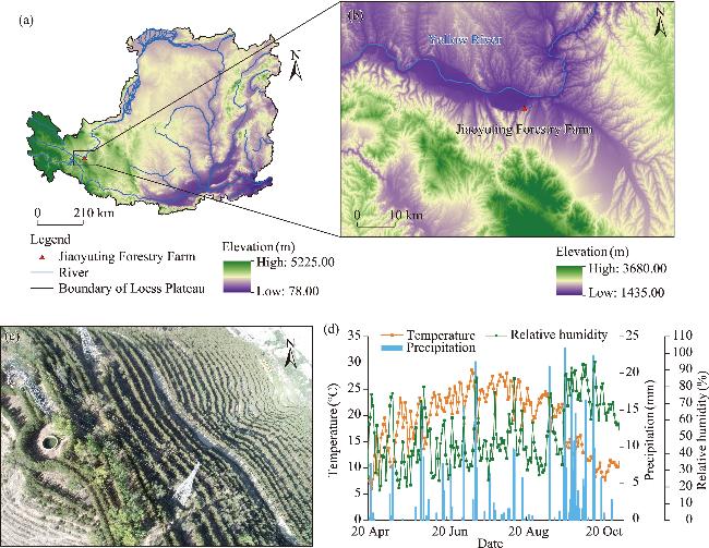
Fig. 1 Geographical location, landscape, and climate of the Jiaoyuting Forestry Farm. (a and b), location of the Jiaoyuting Forestry Farm in the Loess Plateau; (c), unmanned aerial vehicle (UAV) landscape of the Jiaoyuting Forestry Farm; (d), daily temperature, precipitation, and relative humidity during the study period. The flight height of the UAV is 200.00 m.

2.2 Selection of sample plot

We randomly set five plots (S1, S2, S3, S4, and S5; 10.00 m×10.00 m) for forest stand survey (plant height, canopy area, and basal diameter) and soil water measurement in a block of 100.00 m×100.00 m in the Jiaoyuting Forestry Farm. The plant height, canopy area, and basal diameter of each tree in each plot were measured and the average values of each plot were calculated. We randomly selected three sites in each plot to collect soil samples at depth of 0.00-200.00 cm with 20.00 cm intervals (total 10 layers) and dug three soil samples at each layer of each site. The average soil water content of each plot was calculated. Then, according to the measurement results, we selected plot S3, whose vegetation characteristics and soil moisture were nearest to the average values of five plots, as the representative sample plot (Table 1).
Table 1 Information on forest stand survey and soil moisture content
Plot Plant height (m) Canopy area (m2) Basal diameter (m) Soil water content (cm3/cm3)
S1 4.14 4.32 12.04 5.95
S2 4.62 3.06 13.22 7.49
S3 4.96 2.32 13.97 5.90
S4 5.33 2.16 15.89 5.76
S5 5.40 2.00 14.32 5.59
Average 4.89 2.77 13.89 6.14

2.3 Data collection

To observe the meteorological factors of temperature, precipitation, relative humidity, wind speed, and solar radiation, we set a meteorological instrument in the open space outside the forest 100.00 m away from the Jiaoyuting Forestry Farm in the northeastern direction. The monitoring period ranged from 19 April to 31 October, 2023, and the data collection frequency was 30 min.
To obtain highly accurate soil moisture data, we installed a soil water monitor (EJ-200, Jianling Technology Co., Beijing, China) in the representative sample plot. The soil water content at depths of 10.00, 30.00, 50.00, 70.00, 90.00, 110.00, 130.00, 150.00, 170.00, and 190.00 cm in the representative sample plot S3 was monitored in real time from 19 April to 31 October, 2023, with a collecting frequency of 30 min.
We randomly selected three points in the representative sample plot to collect soil samples. In order to ascertain the particle size of soil, we gathered soil samples separately at each sampling point using aluminium boxes, with three parallel samples from each soil layer (consistent with soil water monitoring depth). A total of 90 samples were brought back to the laboratory for air-drying treatment and then passed through a 2.00 mm sieve to manually pick the roots from the soil. The soil was treated with 30.00% hydrogen peroxide and 30.00% hydrochloric acid to remove organic matter and calcium carbonate. Finally, soil particle size was determined using a MS2000 Malvern Laser Particle Sizer (Mastersizer2000-APA2000, Malvern, UK), and particle size values were averaged for each layer of parallel samples (Table 2).
Table 2 Soil physical property at different depths in the Platycladus orientalis (L.) Franco forest
Soil depth (cm) Clay (%) Silt (%) Sand (%) Soil bulk density (g/cm3)
10.00 8.50 70.58 20.93 1.10
30.00 7.90 71.80 20.30 1.12
50.00 8.75 70.19 21.05 1.17
70.00 7.97 70.88 21.15 1.25
90.00 6.45 70.20 23.36 1.19
110.00 6.31 67.92 25.76 1.10
130.00 7.02 67.90 25.08 1.03
150.00 6.28 66.35 27.38 0.94
170.00 6.64 66.69 26.68 1.05
190.00 6.10 66.43 27.48 1.18
We used a ring knife to collect undisturbed soil. The total 90 undisturbed soil samples were collected and brought back to the laboratory in an incubator. The samples were dried at 105.0℃ for 24 h and then weighed. The soil bulk density is the ratio of the dried soil weight to the volume of the ring knife (Table 2).
To obtain the root distribution of the P. orientalis at soil depth of 0.00-200.00 cm, we selected three well-grown P. orientalis trees in the representative sample plot S3 with height, canopy area, and basal diameter close to the average values as representative trees. The roots of three sample trees were collected with a root drill (the drill diameter is 0.08 m) during the vigorous growth period (August 2023). For each tree, three sampling points were established at 120° intervals with a radius of 50.00 cm and centred on the trunk. One sample was taken at 10.00 cm intervals from each sampling point in the 0.00-200.00 cm depth range. Sixty samples were collected from each tree, totalling 180 samples. They were taken back to the laboratory for cleaning. The roots were manually selected and subjected to drying in an oven set at 65.0°C for a period of 48 h. Following this, the roots were weighed on an electronic balance, obtaining the dry weight. The root biomass within each layer was then calculated (Feng et al., 2018; Zhou and Zhao, 2020).
We manually counted the number of leaves on each sample tree and collected leaves from the upper and lower parts of the sample trees in four directions, east, south, west, and north, totalling eight positions per tree. Five leaves were collected from each position, for a total of 120 leaf samples. We used a leaf area analyser (Yaxin1214, LICA United Technology Limited, Beijing, China) to measure the leaf area of each sample tree in each direction, and the average leaf area of a single tree was calculated. The total leaf area was obtained from the number of leaves and the average leaf area of three sample trees, and the ratio of the total leaf area to the area covered by plants was recorded as the leaf area index (Yin et al., 2015; Wang et al., 2020).

2.4 HYDRUS-1D model

The simulation period was from 20 April to 31 October, 2023, and the unit of simulation step was 1.0000 d. The upper boundary was set as an atmospheric boundary to obtain precipitation and infiltration data, and the lower boundary was set as the free infiltration boundary. The 200.00 cm soil profile was divided into 10 layers, and the profile was divided into 200 units at equal intervals of 1.00 cm. Accordingly, 201 nodes and 10 observations were set up. The initial interval was set as 0.0100 d, and the minimum and maximum time intervals were set as 0.0001 and 1.0000 d, respectively.
The parameters involved in HYDRUS-1D model included soil residual water content (Qr), soil saturated water content (Qs), reciprocal of the soil intake value (α), soil pore-size distribution parameter (σ), saturated hydraulic conductivity (Ks), and the pore-connectivity parameter (l). They were obtained by inputting soil particle size and bulk density into the artificial neural network prediction module of HYDRUS-1D model. The obtained parameters were adjusted using the inversion module, and the final values are shown in Table 3.
Table 3 Value of model parameter at different soil depths
Soil depth (cm) Qr (cm3/cm3) Qs (cm3/cm3) α (/cm) σ Ks (cm/d) l
10.00 0.0585 0.3210 0.0038 1.1860 90.80 0.5
30.00 0.0657 0.4770 0.0041 1.3590 122.40 0.5
50.00 0.0695 0.3260 0.0040 1.2225 100.04 0.5
70.00 0.0723 0.3740 0.0044 1.2230 76.61 0.5
90.00 0.0723 0.3280 0.0042 1.1784 107.29 0.5
110.00 0.0745 0.3570 0.0039 1.2358 152.43 0.5
130.00 0.0687 0.3790 0.0036 1.2310 189.56 0.5
150.00 0.0669 0.3990 0.0040 1.2276 157.50 0.5
170.00 0.0698 0.4010 0.0041 1.2354 180.31 0.5
190.00 0.0752 0.4270 0.0039 1.2431 112.95 0.5

Note: Qr, soil residual water content; Qs, soil saturated water content; α, reciprocal of the soil intake value; σ, soil pore-size distribution parameter; Ks, saturated hydraulic conductivity; l, pore-connectivity parameter.

2.4.1 Parameter sensitivity analysis

The sensitivity of each model parameter was analyzed theoretically by single factor perturbation analysis. We set up and down perturbations with 10.00% step size based on the actual input parameters. With the simulated soil water content at 10.00 cm as the output result, the average change rate of the simulation results under different parameter perturbations was calculated, and the influence of parameter changes on the simulation results was analyzed (Huo and Jin, 2017; de Pue et al., 2019).

2.4.2 Moisture transport module

Soil moisture predominantly moves in the vertical direction. Thus, only one-dimensional vertical transport was considered and horizontal and lateral soil moisture flows were ignored. Moreover, the ground was taken as the origin of the coordinates, and the Z-axis downwards direction was chosen as the positive direction. The basic equation for one-dimensional saturated-unsaturated zone soil moisture transport is shown as follows (Šimůnek et al., 2018):
$\frac{\partial \theta }{\partial t}=\frac{\partial }{\partial z}\left[ K \left( \theta \right)\left( \frac{\partial h}{\partial z} \right)+1 \right]-S\left( z,t \right)$,
where θ is the soil water content (cm3/cm3); t is the time (d); z is the soil depth (cm); K(θ) is the unsaturated infiltration coefficient (mm/d); h is the pressure head (cm); and S(z, t) is the water absorption rate of plant roots (cm/d).

2.4.3 Determination of soil kinetic parameters

The soil moisture characteristic curve is fitted to soil water content as a function of soil water suction using the van Genuchten model, which is represented as follows (van Genuchten, 1980):
$K\left( \theta \right)={{K}_{s}}S_{e}^{l}{{\left[ 1-{{\left( 1-S_{e}^{\frac{1}{m}} \right)}^{m}} \right]}^{2}}$,
$\theta \left( h \right)=\left\{ \begin{matrix} {{Q}_{r}}+\frac{{{Q}_{s}}-{{Q}_{r}}}{{{\left( 1+{{\left| \alpha h \right|}^{\sigma }} \right)}^{m}}} \\ {{Q}_{s}}, (h\ge 0) \\ \end{matrix} \right., (h<0)$,
${{S}_{e}}=\frac{\theta -{{Q}_{r}}}{{{Q}_{s}}-{{Q}_{r}}}$,
$m=\frac{1}{1-\sigma }$,
where Qr is the soil residual water content (cm3/cm3); Qs is the soil saturated water content (cm3/cm3); α is the reciprocal of the soil intake value (/cm); σ is the soil pore-size distribution parameter; l is the pore-connectivity parameter; m is the parameter in the soil water retention function; Ks is the saturated hydraulic conductivity (cm/d); θ(h) is the soil water retention curve; and Se is the effective saturation.

2.4.4 Root water uptake module

We numerically resolved the water absorption rate of plant roots S(z, t) using the Feddes model based on the water potential difference, and the calculation is as follows (Šimůnek et al., 2018):
$S\left( z,t \right)=\alpha \left( h \right)\gamma \left( z \right){{T}_{p}}$,
where Tp is the potential transpiration (mm); r(z) is the root water uptake distribution function; and α(h) is the water stress function, which is described using the s-shaped description (Šimůnek et al., 2018):
$\alpha \left( h \right)=\frac{1}{1+{{\left( \frac{h}{{{h}_{50}}} \right)}^{p}}}$,
where h50 is the soil water potential when the potential transpiration decreases by half (cm); and p is a constant.

2.4.5 Calculation of ETp

Based on the Penman-Monteith equation, we calculated ETp using the following formula (Okkan et al., 2024):
$\text{ETp}=\frac{1}{\lambda }\left[ \frac{\Delta \left( {{R}_{n}}-G \right)+{{\rho }_{a}}{{C}_{\rho }}\left( \frac{{{e}_{s}}-{{e}_{a}}}{{{r}_{a}}} \right)}{\Delta +r\left( 1+\frac{{{r}_{s}}}{{{r}_{a}}} \right)} \right]$,
where ETp is the sum of vegetation transpiration and soil evaporation under adequate water supply conditions (mm); λ is the latent heat of vaporization of water (MJ/kg); Rn is the net solar radiation (MJ/(m2•d)); G is the soil heat flux (MJ/(m2•d)); ρa is the average atmospheric density (kg/m3); Cρ is the constant-pressure specific heat capacity of air (J/(kg•°C)); es is the saturation vapor pressure (kPa/°C); ea is the actual water vapor pressure (kPa/°C); r is the wet-dry table constant (kPa/°C); Δ is the gradient of the saturated vapor pressure as a function of temperature (kPa/°C); ra is the aerodynamic impedance (s/m); and rs is the surface impedance (s/m).
Among these, the surface and aerodynamic impedances are related to the vegetation type and growth conditions, and they can be calculated as follows (Okkan et al., 2024):
${{r}_{s}}=\frac{200}{LAI}$,
${{r}_{a}}=\frac{\ln \left[ \frac{{{z}_{m}}\frac{2{{h}_{v}}}{3}}{0.123{{h}_{v}}} \right]\ln \left[ \frac{{{z}_{h}}\frac{2{{h}_{v}}}{3}}{0.123{{h}_{v}}} \right]}{{{0.41}^{2}}{{\mu }_{z}}}$,
where LAI is the leaf area index; zm and zh are the heights from the ground for wind speed and humidity measurements, respectively (m); μz is the wind speed at the height of z (m/s); and hv is the average height of vegetation (m).
We calculated potential evaporation (Ep) and potential transpiration (Tp), according to Beer's law (Šimůnek et al., 2018).
${{\text{T}}_{p}}=\text{E}{{\text{T}}_{p}}\left( 1-{{e}^{-k\text{LAI}}} \right)$,
${{\text{E}}_{p}}=\text{E}{{\text{T}}_{p}}{{e}^{-k\text{LAI}}}$,
where Ep is the potential evaporation (mm); k is an extinction coefficient for global solar radiation; and e is the natural constant. According to White et al. (2000), the k of P. orientalis is 0.51, so we took 0.51 as the value of k in this study.

2.4.6 Calculation of ETa

The ETa was estimated as the sum of actual evaporation (Ea) and actual transpiration (Ta). The calculation formulas are as follows (Šimůnek et al., 2018; Diongue et al., 2022):
${{\text{T}}_{\text{a}}}={{T}_{\text{p}}}\int_{0}^{z}{\alpha (h)\gamma (z)dz}$,
${{E}_{a}}=-K(\frac{\partial h(z,t)}{\partial z}+1)$,
$K={{K}_{s}}S_{e}^{\frac{2}{\sigma }+l+2}$,
where ETa is the actual evapotranspiration (mm); Ta is the actual transpiration (mm); and K is the unsaturated soil hydraulic conductivity.

2.5 Water balance calculation

No runoff occurred in the area, and the formula for the variation of soil water storage (ΔW) obtained from the water balance equation is as follows:
$\Delta W=P+I+{{G}_{r}}E{{T}_{a}}{{D}_{r}}$,
where ΔW is the variation of soil water storage (mm); P is the amount of precipitation (mm); Gr is the upward recharge of deep soil water below rhizosphere (mm); I is the amount of irrigation (mm), obtained from the irrigation record of the Jiaoyuting Forestry Farm; and Dr is the deep percolation (mm). The Gr and Dr were derived from the water flux iteratively fitted by the water movement module in HYDRUS-1D model. If the water flux at 200.00 cm is positive, the value of water flux is regarded as Gr; and if it is negative, the value of water flux is regarded as Dr (Beyene, 2018).

2.6 Evaluation of model accuracy

The model accuracy was evaluated by comparing the fit between the simulated and observed values of soil water content at different depths, and the fitting effect was quantitatively evaluated using the root mean square error (RMSE) and the coefficient of determination (R2):
${{R}^{2}}=1\frac{\sum\limits_{i=1}^{n}{{{\left( {{x}_{i}}{{y}_{i}} \right)}^{2}}}}{\sum\limits_{i=1}^{n}{{{\left( {{x}_{i}}\overline{x} \right)}^{2}}}}$,
$\text{RMSE}=\sqrt{\frac{\sum\limits_{i=1}^{n}{{{\left( {{x}_{i}}-{{y}_{i}} \right)}^{2}}}}{n}}$,
where xi is the measured value; yi is the simulated value; $\overline{x}$ is the average of measured values; and n is the number of samples. According to literature, for the soil moisture simulation of farmland and wetland system, RMSE value of below 0.0300 and R2 value of above 0.5000 actually reflect the soil moisture condition and dynamic characteristics (Galleguillos et al., 2017; Er-Raki et al., 2021).

2.7 Correlation analysis

In order to research the influence of environmental factors on ETa, we adopted the correlation coefficient method and principal component analysis (PCA) method to analyze the correlation between environmental factors and ETa, and utilized the Pearson correlation analysis to obtain the correlation coefficient.

3 Results

3.1 Model test and parameter sensitivity analysis

The observations and the simulation results by HYDRUS-1D model of soil water dynamic changes from 20 April to 31 October 31, 2023, showed that the soil water content significantly fluctuated under the interference of external conditions at depth of 10.00-50.00 cm, while it relatively gently fluctuated with a significant delay at depth of 70.00-190.00 cm. Figure 2 depicts the comparison between the simulated and observed soil water content. Overall, the soil water content in the study area ranged from 0.1266 to 0.2617 cm3/cm3, and the simulated and observed soil water content values in a fixed period of time roughly exhibited the same state of change, with a difference of 0.0003-0.0900 cm3/cm3. The difference mainly occurred due to the uncertainty of model input data. The error was small and within the acceptable range.
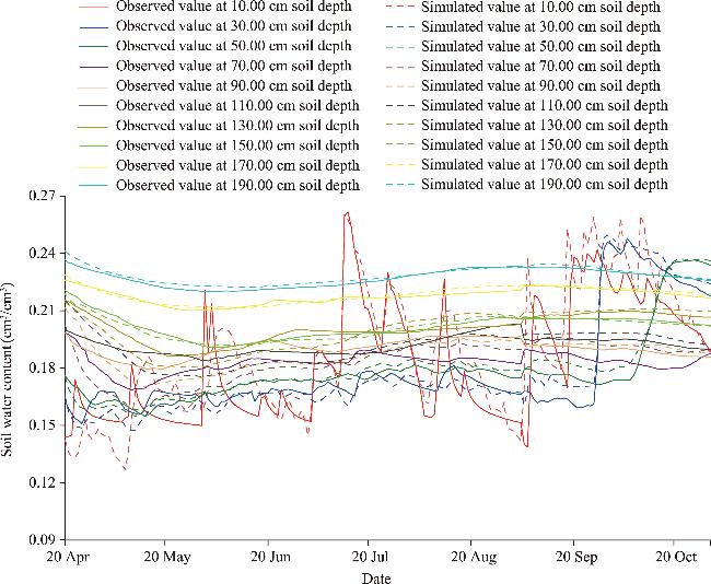
Fig. 2 Comparison of simulated and observed values of soil water content
Moreover, different indices were adopted to evaluate the simulation accuracy of the model (Table 4), the variation range of RMSE for the simulation effect of soil water content was 0.0015-0.0188, which was below 0.0300, and the variation range of R2 was 0.5036-0.9604, which was over 0.5000. Thus, the simulated values obtained in this study were appropriate, and the model was used for simulating the water balance in the artificial P. orientalis forest.
Table 4 Statistic results of simulation verification
Statistic index Soil depth (cm)
10.00 30.00 50.00 70.00 90.00 110.00 130.00 150.00 170.00 190.00
R2 0.7186 0.9604 0.9706 0.6023 0.5036 0.6843 0.8394 0.9326 0.9069 0.9458
Root mean square error (RMSE) 0.0188 0.0060 0.0038 0.0074 0.0066 0.0058 0.0052 0.0016 0.0015 0.0017
Through the sensitivity analysis of parameters, it is found that parameter fluctuations significantly influenced the simulation results (Table 5). Since when the σ perturbation was set to -20.00% and -30.00%, the value of σ was less than 1.0000, out of its range of values, and thus, only fourth-order perturbations were present in the diagram (Fig. 3). The Qs exhibited a high degree of consistency when the perturbation was 20.00% and 30.00%, and their simulated values were lapped in the graph (Fig. 3). The α yielded the same result when the disturbance was -10.00% and 30.00%, with an overlap on Figure 3. The Qs and σ had the greatest influence on the simulation results, and the ranges of change rate of simulation results influenced by Qs and σ were from -28.58% to -19.98% and from -49.92% to -57.33%, respectively (Fig. 3). The Ks and l had little influence on simulation results. The rank of the degree of influence on the simulation results was σ>Qs>Qr>α>Ks>l (Fig. 3).
Table 5 Average change rate of simulation results under different parameter perturbations
Model parameter Change rate of soil water content (%)
D(10.00%) D(20.00%) D(30.00%) D(-10.00%) D(-20.00%) D(-30.00%)
Qr 1.10 2.16 3.27 -1.07 -2.06 -3.15
Qs 7.56 15.06 15.06 -7.87 -14.89 -23.21
α -0.48 -0.94 -1.35 -1.35 1.47 2.49
σ -17.46 -29.02 -36.57 31.51 - -
Ks -0.19 -0.38 -0.42 0.22 0.51 0.77
l 0.10 0.18 0.24 -0.13 -0.20 -0.31

Note: D(10.00%), D(20.00%), D(30.00%), D(-10.00%), D(-20.00%), and D(-30.00%) mean that the disturbance degree is 10.00%, 20.00%, 30.00%, -10.00%, -20.00%, and -30.00%, respectively. The positive value represents that the simulation results become larger under disturbance, and the negative value represents that the simulation results become smaller under disturbance. Due to the limitation of parameter value range, perturbation degree of σ cannot set to -20.00% and -30.00%.

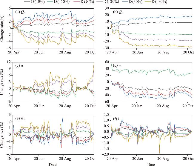
Fig. 3 Change rate of simulation results under different parameter perturbations. (a), Qr; (b), Qs; (c), α; (d), σ; (e), Ks; (f), l. Qr, soil residual water content; Qs, soil saturated water content; Ks, saturated hydraulic conductivity; α, reciprocal of the soil intake value; σ, soil pore-size distribution parameter; l, pore-connectivity parameter. The change rates of simulation results were same when the perturbation degree of Qs was at 20.00% and 30.00%, so the Figure 3b only shows five perturbations. The change rates of simulation results were same when the perturbation degree of α was at -10.00% and 30.00%, so the Figure 3c also shows five perturbations. Due to the limitation of parameter value range, perturbation degree of σ cannot set to -20.00% and -30.00%, the Figure 3d only shows four perturbations.

3.2 Calculation of water balance

In this study area, soil water accumulation items included precipitation, irrigation, water recharge from deep layer, while water consumption items included deep percolation and ETa (Fig. 4). Table 6 illustrates that soil water storage increased by 49.64 mm throughout the simulation period. The negative values of ΔW in May, June, July, and August, indicated that soil water was deficient, due to high water uptake by vegetative root system during this period. The positive values of ΔW in April, September, and October indicated that soil water was surplus, due to weak evapotranspiration in April and low temperatures and persistent precipitation events in September and October. During the simulation period, the cumulative precipitation was 361.00 mm, and total amount of irrigation was 28.60 mm, which was concentrated in July and August. Precipitation was mainly concentrated in July, August, September, and October, accounting for 78.73% of the total precipitation, and precipitation infiltration was the main source of soil moisture in this area. The total upward recharge of deep soil was 315.26 mm, with the highest occurring in September (75.54 mm) and October (93.41 mm).
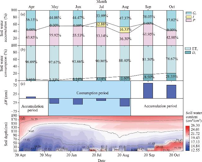
Fig. 4 Soil water budget and dynamic changes simulated by HYDRUS-1D model. (a), soil water accumulation; (b), soil water consumption; (c), variation of soil water storage (ΔW); (d), change of soil water content. P, amount of precipitation; Gr, upward recharge of deep soil water below the rhizosphere; I, amount of irrigation; ETa, actual evapotranspiration; Dr, deep percolation.
Table 6 Soil water balance of the P. orientalis forest from April to October in 2023
Month P (mm) I (mm) Gr (mm) Dr (mm) ETa (mm) ΔW (mm)
April 12.40 0.00 15.88 0.75 18.39 9.13
May 30.20 0.00 23.81 1.93 80.93 -28.85
June 34.20 0.00 27.39 5.92 90.61 -34.94
July 59.00 14.30 37.74 11.22 111.53 -11.71
August 31.80 14.30 41.49 15.39 117.23 -45.03
September 123.00 0.00 75.54 20.89 92.03 85.62
October 70.40 0.00 93.41 18.85 69.54 75.42
Total 361.00 28.60 315.26 74.95 580.27 49.64

Note: ETa, actual evapotranspiration; P, amount of precipitation; I, amount of irrigation; Gr, upward recharge of deep soil water below the rhizosphere; Dr, deep percolation; ΔW, variation of soil water storage. The positive value of ΔW represents that soil water is in surplus, and the negative value represents that soil water is deficient.

According to the simulation results, the total ETa during the simulation period was 580.27 mm, accounting for 88.56% of the total consumption of soil water (Table 6). The highest ETa occurred in July (111.53 mm) and August (117.23 mm), and the overall pattern from April to October exhibited an increasing and then decreasing trend. The deep percolation was another reason for the depletion of soil water. It was 74.95 mm during the simulation period and displayed an overall increasing trend from April to October, which was related to precipitation, the physical properties of soil itself and the water absorption degree of vegetation roots. In conclusion, during the simulation period, the total soil water accumulation was 704.86 mm and the total consumption was 655.22 mm, signifying soil water storage of 49.64 mm.

3.3 Changes in evapotranspiration

According to the simulation results, the total cumulative ETp from 20 April to 31 October, 2023, was 809.67 mm (Fig. 5), which was divided into Ep (95.07 mm) and Tp (714.60 mm). Moreover, the total ETa was 580.27 mm, which was divided into Ea (68.27 mm) and Ta (512.00 mm). On a monthly scale, ETp, Ep, Tp, ETa, Ea, and Ta all displayed a tendency of first increase and then decrease. The ETp, Tp, ETa, and Ta were the highest in August, with values of 179.47, 167.25, 117.23, and 108.42 mm, respectively, and Ep and Ea were the highest in June, with values of 20.31 and 14.62 mm, respectively. Overall, ETp, Tp, ETa, and Ta were higher in July and August compared with the other months. Data were only present for 10.0000 d of April; thus, ETp, Ep, Tp, ETa, Ea, and Ta were low in April; except April, October exhibited the lowest values. On a daily scale, ETp, Ep, Tp, ETa, Ea, and Ta all considerably fluctuated (Fig. 5), but still showed an overall trend of first increase and then decrease. The fluctuations of ETp and Tp as well as ETa and Ta were consistent on the monthly and daily scale. The high average of Tp/ETp (0.87) and Ta/ETa (0.88) indicated that the evapotranspiration in the P. orientalis artificial forest was dominated by transpiration.
Fig. 5 Dynamic change of evapotranspiration on the monthly (a and b) and daily (c and d) scales. ETp, potential evapotranspiration; Ep, potential evaporation; Tp, potential transpiration; Ea, actual evaporation; Ta, actual transpiration.

3.4 Relationship between ETa and ETp

The ETp, which describes the capacity of the atmosphere to absorb surface water through evaporation and transpiration, is roughly comparable to ETa under unrestricted surface water supply conditions. Correlation analysis showed that the R2 of ETa and ETp were 0.9696 and 0.9635 on the monthly and daily scales, respectively (Fig. 6), signifying that ETa and ETp were significantly positively correlated on the monthly and daily scales (P<0.05).
Fig. 6 Relationship between ETp and ETa on the monthly (a) and daily (b) scales. The light blue area that is symmetric on both sides of function represents the 95% confidence interval.
The ratio of ETa/ETp provides the water availability in terrestrial ecosystems and can be used to assess the degrees of drought and water stress to plants. An ecosystem has sufficient water supply when the ratio of ETa/ETp is close to 1.00; and the lower the ratio of ETa/ETp, the greater the water deficit or drought in the ecosystem. In this study, the ratio of ETa/ETp was calculated on the monthly and daily scales and was about 0.72 throughout the simulation period, showing an overall trend of decreasing and then increasing (Fig. 7). On the monthly scale, the average ratio of ETa/ETp was 0.74, the maximum ratio of ETa/ETp was in April (0.84), and the minimum ratio was in August (0.65), indicating that the moisture deficit was most severe in August.
Fig. 7 Variation of ETa/ETp on the monthly (a) and daily (b) scales
On the daily scale, ETa/ETp significantly fluctuated in a short period of time, with maximum of 0.91 and 0.95 on 12 July and 13 July, respectively, which were significantly higher than the average value of 0.68 for July. A sudden change of ETa/ETp was observed at these days, while precipitation on 12 July and 13 July were 21.60 and 7.20 mm, respectively. This indicated that the soil water recharge was sufficient and the P. orientalis was suffering from a low degree of water stress. From 14 June to 5 September, ETa/ETp was generally low. The average ratio of ETa/ETp for this period (0.66) was lower than the average of the entire simulation period (0.75) on the daily scale, indicating that the plants suffered severe water stress from 14 June to 5 September.

3.5 Influence of environmental factors on ETa

The ETa is influenced by many factors. This study investigated the effects of meteorological factors and soil water content at the soil depth of 10.00 cm on ETa dynamics using two methods: PCA and correlation coefficient method. The meteorological indicators considered by this study included temperature, relative humidity, precipitation, wind speed, and solar radiation.
The results of PCA demonstrated that there were significant differences in the extent to which the changes of environmental factors in different months during the growing season of P. orientalis influenced ETa (Fig. 8). In April, which is the dormant period of plants, the response of ETa to environmental factors was not evident. In May and June, temperature, solar radiation, and wind speed were the key factors affecting ETa. In July, the contributions of all five environmental factors to ETa reached their maxima. In August, the contributions of temperature, solar radiation, and wind speed to ETa increased compared with those in July. In September, relative humidity, precipitation, and soil water content were the key factors affecting ETa. In October, relative humidity and precipitation were the key factors affecting ETa.
Fig. 8 Principal component analysis (PCA) diagram of influence factors of ETa. The ellipse represents 95.00% confidence ellipse, and its color is same with the points of the same month. PC, principal component.
On the daily scale, temperature, solar radiation, and wind speed were significantly positively correlated with ETa, with the rank of correlation coefficient being temperature>wind speed>solar radiation (Fig. 9). The relative humidity and precipitation were negatively correlated with ETa. The soil water content at the depth of 10.00 cm did not pass the significance test and the correlation coefficient was small (-0.01).
Fig. 9 Correlation analysis between ETa and environmental factors on the daily scale. (a), temperature; (b), relative humidity; (c), precipitation; (d), solar radiation; (e), wind speed; (f), soil water content. The light blue area that is symmetric on both sides of function represents the 95% confidence interval.

3.6 Influence of environmental factors on ETa/ETp

The ratio of ETa/ETp significantly fluctuated due to the dynamic effects of environmental factors. And the impact of environmental factors on ETa/ETp varied on different time scales (Fig. 10). On both monthly and daily scales, ETa/ETp was negatively correlated with temperature, solar radiation, and wind speed. On the monthly scale, the rank of correlation between temperature, solar radiation, and wind speed and ETa/ETp was temperature>wind speed>solar radiation. The correlation degree of temperature, solar radiation and wind speed on the daily scale was temperature>solar radiation>wind speed. Soil water content, relative humidity, and precipitation were positively correlated with ETa/ETp on different time scales, and the correlation degree was relative humidity>precipitation>soil water content. On the monthly scale, principal component 1 (PC1) was 57.32%, principal component 2 (PC2) was 35.54%, and the contribution of both reached 92.86%; on the daily scale, PC1 was 54.31%, PC2 was 16.32%, and the contribution of both reached 70.63%, signifying that the selected environment factors were representative and reasonable.
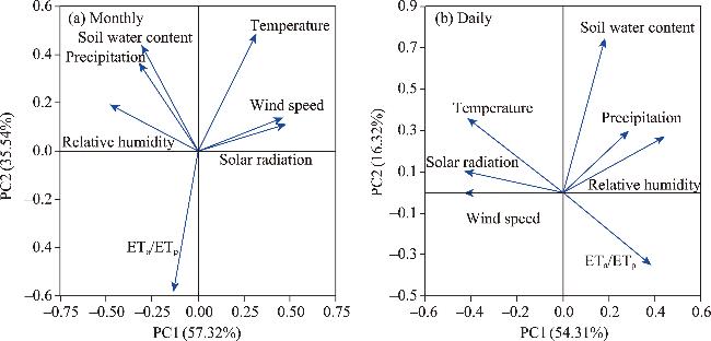
Fig. 10 PCA load diagram of influence factors of ETa/ETp on the monthly (a) and daily (b) scales

4 Discussion

4.1 Assessment of model accuracy and water balance analysis

In the model simulation process, parameter determination is particularly important, and parameter variations significantly impact simulation results (Diongue et al., 2022; Zhou et al., 2022). Graham et al. (2018) investigated four methods of soil hydraulic parameterization and found that measuring soil physical property data to fit model parameters is the best method. Thus, this study utilized measured soil physical property data (soil particle size and soil bulk density) for parameter fitting and subsequently inversion. The high sensitivity factors in this study were σ and Qs (Fig. 3), and more attention should be paid to the accurate grasp of these two factors in subsequent studies.
The HYDRUS-1D model estimates evapotranspiration like water balance models but does not consider the physical processes within the system. Treating the system as a whole, the applicability of this model to the ecosystem can be assessed by validating one of the results (Beyene et al., 2018). Therefore, this study employed the observed and simulated soil water content to evaluate the model accuracy (Han et al., 2015; Zhou et al., 2021). According to the results, April, September, and October were the periods of accumulation. Since the plant growth period had just commenced in April, the root water uptake was not considered to be large. On the other hand, in September and October, continuous precipitation resulted in a large recharge of soil water and the root water uptake simultaneously started to decrease in these two months, which leaded to soil water accumulation.

4.2 Changes in ETa and influence factors

The overall pattern from April to October exhibited an increase firstly and then a decrease, and ETa and Ta in July and August were higher than those in the other months due to higher temperature and solar radiation, which is consistent with the results of Wegehenkel and Beyrich (2014), while Ea in June was higher because the temperature was high and the planting coverage did not reach the most vigorous stage in June. Segmentation of ETa showed that Ta/ETa was 0.88 during the simulation period, while Wolf et al. (2024) concluded that Ta/ETa in arborvitae forests ranged from 0.67 to 0.74. Compared with the results of Wolf et al. (2024), the ratio of Ta/ETa obtained herein was large because our study was conducted in the vigorous period of plant growth rather than all year round. This study simulated the period from April to October, which is the growing season of P. orientalis, and Ta values in these months were higher than those in the other months. D'Acunha et al. (2024) concluded that ETa significantly differed under different land covers. They also stated that in forests ecosystems, Ta does not significantly change throughout the year; whereas significant seasonal variations in Ta were observed in this study because the water-heat combinations in this study area had obvious seasonal variation characteristics. The study area of D'Acunha et al. (2024) is an Amazonian tropical forest, with high temperature and precipitation throughout the year, adequate soil moisture supply, and no obvious seasonal differences in water-heat combinations. However, the study area of this study is located in a semi-arid area with a typical temperate continental climate, with obvious seasonal variations. The study area experiences obvious seasonal Ta variations due to the influence of climatic factors (Li et al., 2020; Liu et al., 2022).
The correlation between ETa and environmental factors has been studied. On a monthly scale, it was found that the degree of influence of environmental factors on ETa varies in different months (Fig. 8). In April, the temperature is relatively low, the evapotranspiration of P. orientalis is at a low level, and the land surface is in a frozen-soil state, so the effect of environmental factors on ETa is not obvious. May is the early stage of the plant growth season. The gradual increase in temperature, the enhancement of solar radiation, and the windy weather keeps the leaf surface of P. orientalis at a relatively low humidity. These reasons lead to the intensification of photosynthesis of P. orientalis and an increase in ETa. Therefore, temperature, solar radiation, and wind speed are the main factors affecting ETa in May. In June, July, and August, with the gradual rise in temperature and the increase in precipitation, consequently solar radiation and relative humidity also increase, and each environmental factor accounts for a relatively large proportion of influence on ETa. In September and October, the precipitation frequency in the study area is relatively high and the temperature decreases, so precipitation and relative humidity are the dominant factors of ETa.
On a daily scale, temperature is a key factor affecting ETa. Guo et al. (2023) concluded that energy is the dominant factor influencing evapotranspiration in the Loess Plateau, net solar radiation is the main factor affecting evapotranspiration, and temperature indirectly affects evapotranspiration through net solar radiation. Hence, the correlation between temperature and evapotranspiration is relatively weak. Since solar radiation data used herein were gross radiation, the results slightly differed from the results of Guo et al. (2023). No consideration of net solar radiation was given in Liu et al. (2022), who considered temperature as the first decisive contributor to evapotranspiration, which is consistent with the results of this study. Galleguillos et al. (2017) showed that ETa has no significant correlation with soil depth, soil texture, and water table conditions. Wu et al. (2022) found that soil water content affects ETa by influencing canopy resistance; however, no significant correlation was found between soil water content and ETa in our study (Fig. 9), which may be due to the fact that the use of soil water content at a depth of 10.00 cm weakened the correlation.

4.3 Correlation between ETa and ETp

Su et al. (2021) showed that ETa and ETp are significantly correlated, and ETa will increase with ETp increasing. The analysis of the simulation results in this study denoted that the change trends of ETa and ETp are consistent. The correlation analysis at monthly and daily scales showed the significant positive correlation between the two, with R2 values of 0.9696 and 0.9635, respectively, which is consistent with existing research results (Meza et al., 2023; Kartal, 2024). Liu (2022) developed a nonlinear function to simulate evapotranspiration through soil water-constrained ETp on the daily scale and showed that the accuracy of evapotranspiration simulation using the nonlinear function is higher than that of the linear and complementary relationship methods. Specifically, they found that ETa and ETp show a unimodal change law in the year and a nonlinear relationship under the multi-year time series. Since this study only analyzed the intra-year change relationship in 2023 and did not analysis its multi-year fluctuation pattern and change magnitude, the time scale needs to be subsequently extended to accurately analysis the dynamic relationship between ETa and ETp. Li et al. (2024) studied the characteristics of ETa/ETp change in the Heihe River Basin and found that the rank of the ratio of ETa/ETp is autumn>spring>summer, indicating high temperatures, strong ETa, and severe water deficit in summer decreas the ratio of ETa/ETp, which is basically consistent with the results of the present study. However, in this study, ETa/ETp in spring was slightly greater than that in autumn, which could be related to the vegetation type (Lian et al., 2018; Zhai et al., 2019; Wang et al., 2023). The P. orientalis examined herein is an evergreen tree that even grows in autumn under suitable temperature and water conditions, while the Populus euphratica Oliv. is a deciduous tree with yellow leaves, reduced chlorophyll, and reduced water availability in autumn (Li et al., 2024). Therefore, the ETa/ETp change pattern of poplar slightly differs from that of this study. The ETa/ETp presented a consistent trend on the monthly and daily scales, but large fluctuations were observed on the daily scale, with obvious abrupt changes on 12 May, 13 May, 12 July, and 24 September, which were caused by considerable precipitation. The fluctuations of ETa/ETp were closely related to meteorological factors, with temperature being the dominant factor (Liu et al., 2019).

4.4 Recommendations for management of artificial forest and research perspectives

According to the water balance theory, the degree of water deficit varied from May to August in this study. The plant water use efficiency is usually higher when sufficient water is present rather than that when water is deficit (Zhang et al., 2024). Based on the existing irrigation system, it is necessary to increase irrigation from May to August. In August, the water deficit is most severe and transpiration is most intense. Hence, using August as the main irrigation period for this artificial forest is the most beneficial for plants' growth. The study area is located in northwestern arid area, where evaporation is strong and deep percolation increases in September and October when precipitation is high. Thus, to control soil evaporation and deep percolation, we should adopt the irrigation of small amount for many times. Additionally, P. orientalis trees in the Jiaoyuting Forestry Farm are more than 30 a old, and numerous branches and leaves at the bottom are dead; therefore, cliping dry lateral branches and then covering soil with them is appropriate. The measure of covering the ground with dead branches will not only reduce canopy density, decrease the interception loss of precipitation, and increase the infiltration of precipitation, but also reduce the evaporation loss of soil and improve soil fertility, which is crucial for the growth of P. orientalis.
Moreover, ETa and ETp are influenced by other factors such as vegetation and soil (Yang et al., 2014; Šípek et al., 2020; Yan et al., 2021; Dai et al., 2022; Li et al., 2022). This study only analyzed the characteristics of changes on the monthly and daily scales. Therefore, in future studies, the timescale should be extended to more comprehensively study the variation characteristics of ETp and ETa and their influence factors at different time scales, analyze the characteristics of single peaks and seasonal changes within a year, quantify the contributions of meteorological indicators, leaves, and soil properties, and study the characteristics of ecosystem evapotranspiration dynamics and its influence factors. Additionally, this study only considered the land where a single vegetation is the dominant species. Therefore, the scope should be extended by increasing the number of sampling points to research the evapotranspiration dynamics and influence factors under different land covers, thus improving the regional representativeness.

5 Conclusions

This study utilized HYDRUS-1D model to quantify the soil moisture dynamics and evapotranspiration characteristics of the artificial forest on western Loess Plateau. Calculations showed that the soil water was surplus during the entire simulation period, but according to the plant growth characteristics, the soil water was deficit in May, June, July, and August. The ETp, Ep, Tp, ETa, Ea, and Ta exhibited obvious seasonal change both on the monthly and daily scales. From April to October, the values of ETp, Tp, ETa, and Ta first increased and then decreased, with a peak in August; and the values of Ep and Ea also showed a trend of increase firstly and then decrease, with peak value in June. Analysis showed that evapotranspiration mainly stemmed from transpiration and that ETa was significantly positively correlated with ETp. The ETa was significantly positively correlated with temperature, solar radiation, and wind speed, negatively correlated with relative humidity and precipitation, and not significantly correlated with soil water content. The results showed that HYDRUS-1D model has good applicability in evapotranspiration analysis in arid areas. Based on the results, August is the main irrigation period, and increasing the amount of water input from May to August is essential through irrigation with high frequency and low amount to maintain healthy plant growth. The result provided theoretical reference for water management of artificial forests and deepen the understanding of evapotranspiration and the effects of each influence factor on ETa in arid area. Future studies should strengthen the split research of evapotranspiration under different land covers and extend the time scale to provide a theoretical basis for vegetation restoration and management in large regional arid areas.

Conflict of interest

The authors declare that they have no known competing financial interests or personal relationships that could have appeared to influence the work reported in this paper.

Acknowledgements

This research was financially supported by the National Natural Science Foundation of China (42071047, 41771035), the Basic Research Innovation Group Project of Gansu Province (22JR5RA129), and the Excellent Doctoral Program in Gansu Province (24JRRA152).

Author contributions

Conceptualization: LU Rui, ZHANG Mingjun, ZHANG Yu; Formal analysis and methodology: LU Rui, ZHANG Yu; Data curation: LU Rui, ZHANG Yu, QIANG Yuquan; Writing - original preparation: LU Rui; Funding acquisition: ZHANG Mingjun, QIANG Yuquan; Writing - review and editing: LU Rui, ZHANG Yu, QIANG Yuquan, CHE Cunwei, SUN Meiling, WANG Shengjie. All authors approved the manuscript.
[1]
Beyene A, Cornelis W, Verhoest N E C, et al. 2018. Estimating the actual evapotranspiration and deep percolation in irrigated soils of a tropical floodplain, northwest Ethiopia. Agricultural Water Management, 202: 42-56.

[2]
Cao X H, Zheng Y J, Lei Q L, et al. 2023. Increasing actual evapotranspiration on the Loess Plateau of China: an insight from anthropologic activities and climate change. Ecological Indicators, 157: 111235, doi: 10.1016/j.ecolind.2023.111235.

[3]
Chen D Y, Hu X T, Duan X W, et al. 2023. Incorporating dynamic schemes of canopy light extinction coefficient improves transpiration model performance for fruit plantations. Journal of Hydrology, 627: 130397, doi: 10.1016/j.jhydrol.2023.130397.

[4]
Chen W L, Wang J J, Liu Y F, et al. 2021. Using bromide data tracer and HYDRUS-1D to estimate groundwater recharge and evapotranspiration under film-mulched drip irrigation in an arid inland basin, Northwest China. Hydrological Processes, 35(7): e14290, doi: 10.1002/hyp.14290.

[5]
D'Acunha B, Dalmagro H J, Zanella de Arruda P H, et al. 2024. Changes in evapotranspiration, transpiration and evaporation across natural and managed landscapes in the amazon, cerrado and pantanal biomes. Agricultural and Forest Meteorology, 346: 109875, doi: 10.1016/j.agrformet.2023.109875.

[6]
Dai L C, Fu R Y, Guo X W, et al. 2022. Soil moisture variations in response to precipitation across different vegetation types on the northeastern Qinghai-Tibet Plateau. Frontiers in Plant Science, 13: 854152, doi: 10.3389/fpls.2022.854152.

[7]
de Pue J, Rezaei M, van Meirvenne M, et al. 2019. The relevance of measuring saturated hydraulic conductivity: sensitivity analysis and functional evaluation. Journal of Hydrology, 576: 628-638.

[8]
Diongue D M L, Roupsard O, Do F C, et al. 2022. Evaluation of parameterisation approaches for estimating soil hydraulic parameters with HYDRUS-1D in the groundnut basin of Senegal. Hydrological Sciences Journal, 67(15): 2327-2343.

[9]
Diongue D M L, Stumpp C, Roupsard O, et al. 2023. Estimating water fluxes in the critical zone using water stable isotope approaches in the groundnut and ferlo basins of Senegal. Hydrological Processes, 37(1): e14787, doi: 10.1002/hyp.14787.

[10]
Er-Raki S, Ezzahar J, Merlin O, et al. 2021. Performance of the HYDRUS-1D model for water balance components assessment of irrigated winter wheat under different water managements in semi-arid region of Morocco. Agricultural Water Management, 244: 106546, doi: 10.1016/j.agwat.2020.106546.

[11]
Feng T C, Su T, Ji F, et al. 2018. Temporal characteristics of actual evapotranspiration over China under global warming. Journal of Geophysical Research: Atmospheres, 123(11): 5845-5858.

[12]
Galleguillos M, Jacob F, Prévot L, et al. 2017. Estimation of actual evapotranspiration over a rainfed vineyard using a 1-D water transfer model: A case study within a Mediterranean watershed. Agricultural Water Management, 184: 67-76.

[13]
Gao X R, Zhao Q, Zhao X N, et al. 2017. Temporal and spatial evolution of the standardized precipitation evapotranspiration index (SPEI) in the Loess Plateau under climate change from 2001 to 2050. Science of the Total Environment, 595: 191-200.

[14]
Ge F C, Xu M X, Gong C, et al. 2022. Land cover changes the soil moisture response to precipitation on the Loess Plateau. Hydrological Processes, 36(11): e14714, doi: 10.1002/hyp.14714.

[15]
Graham S L, Srinivasan M S, Faulkner N, et al. 2018. Soil hydraulic modeling outcomes with four parameterization methods: comparing soil description and inverse estimation approaches. Vadose Zone Journal, 17(1): 1-10.

[16]
Guo F N, Liu D F, Mo S H, et al. 2023. Estimation of daily evapotranspiration in gully area scrub ecosystems on Loess Plateau of China based on multisource observation data. Ecological Indicators, 154: 110671, doi: 10.1016/j.ecolind.2023.110671.

[17]
Han M, Zhao C Y, Šimůnek J, et al. 2015. Evaluating the impact of groundwater on cotton growth and root zone water balance using HYDRUS-1D coupled with a crop growth model. Agricultural Water Management, 160: 64-75.

[18]
He Z M, Jia G D, Liu Z Q, et al. 2020. Field studies on the influence of precipitation intensity, vegetation cover and slope length on soil moisture infiltration on typical watersheds of the Loess Plateau, China. Hydrological Processes, 34(25): 4904-4919.

[19]
Huo S Y, Jin M G. 2017. Effect of parameter sensitivity of van Genuchten model on numerical simulation of precipitation recharge. Earth Science, 42(3): 447-452, 470. (in Chinese)

[20]
Jiang F X, Xie X H, Liang S L, et al. 2021. Loess Plateau evapotranspiration intensified by land surface radiative forcing associated with ecological restoration. Agricultural and Forest Meteorology, 311: 108669, doi: 10.1016/j.agrformet.2021.108669.

[21]
Jin Z, Guo L, Lin H, et al. 2018. Soil moisture response to precipitation on the Chinese Loess Plateau after a long-term vegetation rehabilitation. Hydrological Processes, 32(12): 1738-1754.

[22]
Kartal V. 2024. Prediction of monthly evapotranspiration by artificial neural network model development with Levenberg-Marquardt method in Elazig, Turkey. Environmental Science and Pollution Research, 31: 20953-20969.

[23]
Kumar H, Srivastava P, Lamba J, et al. 2023. A methodology to optimize site-specific field capacity and irrigation thresholds. Agricultural Water Management, 286: 108385, doi: 10.1016/j.agwat.2023.108385.

[24]
Li B B, Wang Y Q, Hill R L, et al. 2019. Effects of apple orchards converted from farmlands on soil water balance in the deep loess deposits based on HYDRUS-1D model. Agriculture, Ecosystems and Environment, 285: 106645, doi: 10.1016/j.agee.2019.106645.

[25]
Li B B, Biswas A, Wang Y Q, et al. 2021. Identifying the dominant effects of climate and land use change on soil water balance in deep loessial vadose zone. Agricultural Water Management, 245: 106637, doi: 10.1016/j.agwat.2020.106637.

[26]
Li L J, Song X Y, Xia L, et al. 2020. Modelling the effects of climate change on transpiration and evaporation in natural and constructed grasslands in the semi-arid Loess Plateau, China. Agriculture, Ecosystems and Environment, 302: 107077, doi: 10.1016/j.agee.2020.107077.

[27]
Li L J, Song X Y, Zhao X K, et al. 2022. Modeling the impact of climate change and vegetation conversion on water budget: a case study in the Loess Plateau of China. Journal of Hydrology: Regional Studies, 40: 101040, doi: 10.1016/j.ejrh.2022.101040.

[28]
Li S Y, Zhang D P, Xing Y H, et al. 2024. Interannual dynamics and controlling factors of the ratio of actual to potential evapotranspiration across typical ecosystems within the Heihe River Basin. Hydrological Processes, 38(1): e15073, doi: 10.1002/hyp.15073.

[29]
Li Y Z, Liang K, Bai P, et al. 2016. The spatiotemporal variation of reference evapotranspiration and the contribution of its climatic factors in the Loess Plateau, China. Environmental Earth Sciences, 75: 354, doi: 10.1007/s12665-015-5208-7.

[30]
Lian J J, Li D F, Huang M B, et al. 2018. Evaluation of remote sensing-based evapotranspiration estimates using a water transfer numerical simulation under different vegetation conditions in an arid area. Hydrological Processes, 32(12): 1801-1813.

[31]
Liu Y, Jiang Q, Wang Q Y, et al. 2022. The divergence between potential and actual evapotranspiration: An insight from climate, water, and vegetation change. Science of the Total Environment, 807: 150648, doi: 10.1016/j.scitotenv.2021.150648.

[32]
Liu Y J, Chen J, Pan T. 2019. Analysis of changes in reference evapotranspiration, pan evaporation, and actual evapotranspiration and their influencing factors in the North China Plain during 1998-2005. Earth and Space Science, 6(8): 1366-1377.

[33]
Liu Z F. 2022. Estimating land evapotranspiration from potential evapotranspiration constrained by soil water at daily scale. Science of the Total Environment, 834: 155327, doi: 10.1016/j.scitotenv.2022.155327.

[34]
Lu R, Zhang M J, Zhang Y, et al. 2024. Soil water infiltration of artificial Platycladus orientalis of Nanshan Mountain in Lanzhou under different precipitation and precipitation intensity. Journal of Soil and Water Conservation, 38(2): 364-376. (in Chinese)

[35]
L, Parajuli K, Hipps L E, et al. 2024. Multi-year evapotranspiration estimates from four common vegetation types in a montane region of the intermountain west. Agricultural and Forest Meteorology, 345: 109861, doi: 10.1016/j.agrformet.2023.109861.

[36]
X Z, Zuo Z G, Ni Y X, et al. 2019. Climatic and human-related indicators and their implications for evapotranspiration management in a watershed of Loess Plateau, China. Ecological Indicators, 101: 143-149.

[37]
Meza K, Torres-Rua A F, Hipps L, et al. 2023. Spatial estimation of actual evapotranspiration over irrigated turfgrass using sUAS thermal and multispectral imagery and TSEB model. Irrigation Science, 23: 899, doi: 10.1007/s00271-023-00899-y.

[38]
Okkan U, Fistikoglu O, Ersoy Z B, et al. 2024. Analyzing the uncertainty of potential evapotranspiration models in drought projections derived for a semi-arid watershed. Theoretical and Applied Climatology, 155: 2329-2346.

[39]
Peng S Z, Ding Y X, Wen Z M, et al. 2017. Spatiotemporal change and trend analysis of potential evapotranspiration over the Loess Plateau of China during 2011-2100. Agricultural and Forest Meteorology, 233: 183-194.

[40]
Ramos T B, Liu M H, Paredes P, et al. 2023. Salts dynamics in maize irrigation in the Hetao Plateau using static water table lysimeters and HYDRUS-1D with focus on the autumn leaching irrigation. Agricultural Water Management, 283: 108306, doi: 10.1016/j.agwat.2023.108306.

[41]
Šimůnek J, Šejna M, Saito H, et al. 2018. HYDRUS-1D Manual. [2024-04-23]. https://www.pc-progress.com.

[42]
Šípek V, Hnilica J, Vlček L, et al. 2020. Influence of vegetation type and soil properties on soil water dynamics in the Šumava Mountains. Journal of Hydrology, 582: 124285, doi: 10.1016/j.jhydrol.2019.124285.

[43]
Su T, Feng T C, Huang B C, et al. 2021. Long-term mean changes in actual evapotranspiration over China under climate warming and the attribution analysis within the Budyko framework. International Journal of Climatology, 42(2): 1136-1147.

[44]
Thayalakumaran T, McCaskill M, Morse-McNabb E M. 2018. Estimating soil water in high-precipitation zones under pasture. Agricultural Systems, 165: 252-263.

[45]
van Genuchten M. 1980. A closed-form equation for predicting the hydraulic conductivity of unsaturated soils. Soil Science Society of America Journal, 44(5): 892-898.

[46]
Wang G S, Tang P C, Xu B, et al. 2023. Study on water and heat transport of different types of vegetations and fields in Pengbo alpine irrigation district of Qinghai Tibet Plateau. Journal of Hydrology, 618: 129201, doi: 10.1016/j.jhydrol.2023.129201.

[47]
Wang X F, Li Y, Chau H W, et al. 2020. Reduced root water uptake of summer maize grown in water-repellent soils simulated by HYDRUS-1D. Soil and Tillage Research, 209: 104925, doi: 10.1016/j.still.2020.104925.

[48]
Wegehenkel M, Beyrich F. 2014. Modelling hourly evapotranspiration and soil water content at the grass-covered boundary-layer field site Falkenberg, Germany. Hydrological Sciences Journal, 59(2): 376-394.

[49]
Wegehenkel M, Rummel U, Beyrich F. 2017. Long-term analysis of measured and simulated evapotranspiration and soil water content. Hydrological Sciences Journal, 62(10): 1532-1550.

[50]
White M A, Thornton P E, Running S W, et al. 2000. Parameterization and sensitivity analysis of the BIOME-BGC terrestrial ecosystem model: net primary production controls. Earth Interactions, 4(3): 1-85.

[51]
Wolf S, Paul-Limoges E, Sayler D, et al. 2024. Dynamics of evapotranspiration from concurrent above- and below-canopy flux measurements in a montane Sierra Nevada forest. Agricultural and Forest Meteorology, 346: 109864, doi: 10.1016/j.agrformet.2023.109864.

[52]
Wu Y Q, Song S, Li F D, et al. 2023. Multimedia fate of sulfamethoxazole (SMX) in a water-scarce city by coupling fugacity model and HYDRUS-1D model. Science of the Total Environment, 881: 163331, doi: 10.1016/j.scitotenv.2023.163331.

[53]
Wu Z J, Cui N B, Zhao L, et al. 2022. Estimation of maize evapotranspiration in semi-humid regions of northern China using Penman-Monteith model and segmentally optimized Jarvis model. Jocurnal of Hydrology, 607: 127483, doi: 10.1016/j.jhydrol.2022.127483.

[54]
Xiang K Y, Li Y, Horton R, et al. 2020. Similarity and difference of potential evapotranspiration and reference crop evapotranspiration—a review. Agricultural Water Management, 232: 106043, doi: 10.1016/j.agwat.2020.106043.

[55]
Yan W H, Zhou Q W, Peng D W, et al. 2021. Soil moisture responses under different vegetation types to winter precipitation events in a humid karst region. Environmental Science and Pollution Research, 28: 56984-56995.

[56]
Yang L, Chen L D, Wei W, et al. 2014. Comparison of deep soil moisture in two re-vegetation watersheds in semi-arid regions. Journal of Hydrology, 513: 314-321.

[57]
Yang Z L, Bai P, Li Y Z. 2022. Quantifying the effect of vegetation greening on evapotranspiration and its components on the Loess Plateau. Journal of Hydrology, 613: 128446, doi: 10.1016/j.jhydrol.2022.128446.

[58]
Yi C Q, Fan J. 2016. Application of HYDRUS-1D model to provide antecedent soil water contents for analysis of runoff and soil erosion from a slope on the Loess Plateau. Catena, 139: 1-8.

[59]
Yi J, Li H J, Zhao Y, et al. 2022. Assessing soil water balance to optimize irrigation schedules of flood-irrigated maize fields with different cultivation histories in the arid region. Agricultural Water Management, 265: 107543, doi: 10.1016/j.agwat.2022.107543.

[60]
Yin L H, Zhou Y X, Huang J T, et al. 2015. Interaction between groundwater and trees in an arid site: Potential impacts of climate variation and groundwater abstraction on trees. Journal of Hydrology, 528: 435-448.

[61]
Zhai L, Wang X, Wang P, et al. 2019. Vegetation and location of water inflow affect evaporation in a subtropical wetland as indicated by the deuterium excess method. Ecohydrology, 12(4): e2082, doi: 10.1002/eco.2082.

[62]
Zhang Y, Zhang M J, Qiang Y Q, et al. 2024. Estimating non-productive water losses in irrigated Platycladus orientalis plantations in semi-arid mountainous: Based on stable isotopes. Science of the Total Environment, 934: 173279, doi: 10.1016/j.scitotenv.2024.173279.

[63]
Zhou H, Zhao W Z. 2020. Mechanisms of soil moisture availability in vadose zone of a sand dune system: Linking soil physical properties and precipitation patterns. Water and Environment Journal, 34(S1): 139-157.

[64]
Zhou T T, Šimůnek J, Braud I, et al. 2021. Adapting HYDRUS-1D to simulate the transport of soil water isotopes with evaporation fractionation. Environmental Modelling and Software, 143: 105118, doi: 10.1016/j.envsoft.2021.105118.

[65]
Zhou T T, Šimůnek J, Braud I, et al. 2022. The impact of evaporation fractionation on the inverse estimation of soil hydraulic and isotope transport parameters. Journal of Hydrology, 612: 128100, doi: 10.1016/j.jhydrol.2022.128100.

文章导航

/