• Arash TAFTEH , * ,
  • Mohammad R EMDAD ,
  • Azadeh SEDAGHAT
展开

收稿日期: 2024-06-30

  修回日期: 2024-11-09

  录用日期: 2024-11-27

  网络出版日期: 2025-08-12

Improving irrigation management in wheat farms through the combined use of the AquaCrop and WinSRFR models

  • Arash TAFTEH , * ,
  • Mohammad R EMDAD ,
  • Azadeh SEDAGHAT
Expand
  • Department of Irrigation and Soil Physics, Soil and Water Research Institute, Agricultural Research Education and Extension Organization (AREEO), Karaj 31587-77871, Iran
*Arash TAFTEH (E-mail: )

Received date: 2024-06-30

  Revised date: 2024-11-09

  Accepted date: 2024-11-27

  Online published: 2025-08-12

本文引用格式

Arash TAFTEH , Mohammad R EMDAD , Azadeh SEDAGHAT . [J]. Journal of Arid Land, 2025 , 17(2) : 245 -258 . DOI: 10.1007/s40333-025-0005-y

Abstract

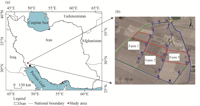
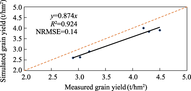
Water is essential for agricultural production; however, climate change has exacerbated drought and water stress in arid and semi-arid areas such as Iran. Despite these challenges, irrigation water efficiency remains low, and current water management schemes are inadequate. Consequently, Iranian crops suffer from low water productivity, highlighting the urgent need for enhanced productivity and improved water management strategies. In this study, we investigated irrigation management conditions in the Hamidiyeh farm, Khuzestan Province, Iran and used the calibrated AquaCrop and WinSRFR (a surface irrigation simulation model) models to reflect these conditions. Subsequently, we examined different management scenarios using each model and evaluated the results from the second year. The findings demonstrated that combining simulation of the AquaCrop and WinSRFR models was highly effective and could be employed for irrigation management in the field. The AquaCrop model accurately simulated wheat yield in the first year, being 2.6 t/hm2, which closely aligned with the measured yield of 3.0 t/hm2. Additionally, using the WinSRFR model to adjust the length of existing borders from 200 to 180 m resulted in a 45.0% increase in efficiency during the second year. To enhance water use efficiency in the field, we recommended adopting borders with a length of 180 m, a width of 10 m, and a flow rate of 15 to 18 L/s. The AquaCrop and WinSRFR models accurately predicted border irrigation conditions, achieving the highest water use efficiency at a flow rate of 18 L/s. Combining these models increased farmers' average water consumption efficiency from 0.30 to 0.99 kg/m³ in the second year. Therefore, the results obtained from the AquaCrop and WinSRFR models are within a reasonable range and consistent with international recommendations. This adjustment is projected to improve the water use efficiency in the field by approximately 45.0% when utilizing the border irrigation method. Therefore, integrating these two models can provide comprehensive management solutions for regional farmers.

1 Introduction

Water scarcity is a pressing issue in the agriculture of arid and semi-arid areas like Iran, where agriculture is the largest consumer of water. Effective water consumption management is essential, yet water use efficiency in Iranian agriculture remains extremely low. The average irrigation system efficiency in Iran is approximately 35.0% (Madani, 2014), significantly lower than the 70.0%-90.0% efficiency observed in the most developed countries (Nazari et al., 2018). To mitigate Iranian water shortage, conserving water resources and promoting affordable and sustainable irrigation practices are imperative.
Since 1960, the Iranian government has prioritized increasing the productivity of irrigated agriculture (Forouzani and Karami, 2011). Despite increased investments in dam construction, low-interest loans, and policy measures like subsidized agricultural water and energy use, many water management schemes have not yielded satisfactory results (Keshavarz et al., 2013; Madani, 2014). Rapid economic and infrastructural growth in Iran has often overlooked the interrelationships between water, environment, and ecosystem components. This neglect leads to a lack of integrated perspectives on human-natural systems and disregards local realities and legitimacy in water management practices. Assessing site-specific challenges is crucial for sustainable water management (Hjorth and Madani, 2014). Proper irrigation management can achieve high efficiency, leading to reduced operating costs, increased production per unit of consumed water, and environmental benefits through better management (Thebuwena et al., 2024).
Two key factors determine water consumption management and efficiency improvement. The first is fertilizer nutrition, which imposes significant costs on farmers and leads to reluctance among local farmers to adopt it. The second factor, which can be easily controlled in the area, is the increase in water use efficiency. Extensive research has been conducted on determining water use efficiency and its management (Horne et al., 2018; Zhou et al., 2021). Implementing research on the impact of different irrigation management practices and their effects on crop performance requires considerable time and resources. Crop models provide the ability to consider and measure parameters related to water, soil, and plants, making them critical tools for improving water management on farms (Zhai et al., 2022). For example, the AquaCrop model can simulate irrigation needs, and the WinSRFR model can propose irrigation methods (Alavi et al., 2022). The AquaCrop model, based on complex biophysical processes, can simulate and predict performance and water consumption efficiency under different irrigation management conditions (Amirouche et al., 2021).
A review of the AquaCrop model showed that it was validated using observed data collected during the growing season. Model calibration revealed a good fit for canopy cover, and validation results showed a good fit for canopy cover with 100.0% water application during the development and mid-growth seasons of potatoes. The AquaCrop model is simple to use, requires fewer input data, and has high simulation precision, making it a useful tool for forecasting crop yield under deficit irrigation and for water management to increase agricultural irrigation efficiency in data-scarce areas (Wale et al., 2022). The AquaCrop model is highly effective for evaluating irrigation scenarios and has acceptable accuracy in improving irrigation management (Corbari et al., 2021).
Research comparing the AquaCrop, World Food Study (WOFOST), and CropSyst models in simulating sunflower growth showed that the AquaCrop model was preferred due to its simplicity and lower data requirements (Raes et al., 2009). Evaluations of the AquaCrop model in simulating wheat growth in India and eastern Algeria indicated no statistical difference between measured results and simulated values (Guendouz et al., 2014; Kumar et al., 2014). In China, the AquaCrop model's estimation error for dry matter was between 160 and 380 kg/hm2, and for grain yield, the error ranged from 0.5 to 1.4 t/hm2 (Zhang et al., 2013). Investigations using the AquaCrop model to simulate potato yield in Jiroft, Kerman Province, Iran, showed an error of up to 9.0 t in yield simulation (Afshar and Neshat, 2013). These models have been applied in different countries and have shown different results, which could be attributed the fact that each country has unique internal (strengths and weaknesses) and external (opportunities and threats) factors influencing water management (Nazari et al., 2018)
To determine the effects of plot or border dimensions, as well as changes in flow and slope, on water use efficiency and related components, researchers have developed various models. The surface irrigation models (SIRMOD) and WinSRFR (a surface irrigation simulation model) models are among the common practical models used to assess the impact of changes in dimensions (length and width of borders), discharge, slope, and other parameters related to water use efficiency in the field to provide proper irrigation management and improve water use efficiency (Radmanesh et al., 2023). Tafteh and Emdad (2017) investigated water use productivity in Khuzestan Province, Iran, using the WinSRFR model. They stated that the model could be applied to farms using border strip irrigation and accurately estimated water use efficiency in this practice. Moreover, water use productivity rose from 0.61 in the first year to 0.89 in the second year when the model managed border strip irrigation. Taghizadeh et al. (2013) evaluated the WinSRFR model using field data, zero inertia, and kinematic wave methods. The results showed that the model was the most sensitive to inlet flow rate, flow interruption time, and parameters of the infiltration equation. In research optimizing border irrigation dimensions using the WinSRFR model, it was reported that water storage in the soil was about 49 mm, and the best performance was achieved for border irrigation with a length of 200 m and a semi-heavy texture. At least 120 m are needed for high efficiency in the border irrigation method because lengths less than 120 m and widths of 3-5 m increase water use efficiency by 26.0% (Chen et al., 2013).
Considering that the number of irrigation cycles is critical to wheat yield and that water consumption efficiency is low in most wheat field in the area, the capability of the AquaCrop model in simulating wheat yield with irrigation cycles has not been thoroughly investigated. Therefore, in this study, after calibrating the model, we considered scenarios of different irrigation management practices in terms of irrigation intervals (according to the usual number of irrigations in the Hamidiyeh region, Khuzestan Province, Iran) as variables. The effect of irrigation intervals on wheat yield in the Hamidiyeh region was investigated and evaluated to validate the model and provide a suitable irrigation management scenario. Additionally, influential factors were examined to improve water use efficiency on the farm, and the most suitable irrigation scenario was selected and recommended. According to previous research, the length and width of the border, inlet flow, slope, and flow interruption time are the most important parameters affecting water use efficiency in the field (Nie et al., 2014).
In general, the AquaCrop and WinSRFR models have been investigated separately in various studies (Abi Saab et al., 2015; Xu et al., 2019; Mazarei et al., 2020; Corbari et al., 2021), but no study has combined these two models to improve farm water management. As a result, this study provides an algorithm for analyzing the combined results of the two models, which can be used to improve farm water efficiency and productivity. Therefore, we simulated changes in border length, cut-off time, flow rate, water consumption efficiency, and water use efficiency in wheat fields in the Hamidiyeh region using the AquaCrop and WinSRFR models.

2 Materials and methods

2.1 Study area

The study was conducted in the Ramseh village of Hamidiyeh region, Khuzestan Province, Iran (31°04′N, 49°39′E; Fig. 1). The study area has a desert climate, which is excessively hot and dry in the summer. Precipitation is concentrated in the winter, ranging from 300 to 500 mm. Two agricultural years, i.e., 2018-2019 and 2019-2020 and three different plots, each approximately 10 hm2 in size, were selected in the Hamidiyeh region. Sampling, measurements, and determination of soil, water, and plant parameters as well as irrigation management practices required by the AquaCrop model were carried out.
Fig. 1 Location of the study area (a) and farms (b) in the Hamidiyeh region, Iran. D, sluice gate.
Within each 10-hm2 plot, a farm (totalling three farms; Fig. 1), each with an area of approximately 2000 m² (border width of 8-10 m and border length of 150-200 m), was chosen for the collection of soil, water, plant, and irrigation management data. The Chamran wheat variety was used, and planting occurred on 15 November, 2018. Fertilization was applied twice during the tillering and flowering stages, with approximately 150 kg/hm2 of urea fertilizer used at each stage.

2.2 Experimental design

To calibrate the AquaCrop model, we measured and recorded various parameters in the selected fields at different growth stages. These parameters included germination percentage, number of days from planting to emergence, maximum canopy cover, leaf senescence, leaf maturity, length of the flowering period, number of days from planting to flowering, maximum root depth, number of days from planting to reaching maximum root depth, total yield, seed yield, harvest index, and plant dry matter yield.
Based on the results, the key developmental stages of wheat in the Hamidiyeh region occurred on the following dates: germination on 27 November, tillering on 20 December, stem elongation on 22 January, flowering on 25 February, seed filling on 20 March, and ripening on 25 April of the following year. Table 1 presents the physical and chemical characteristics of the soils in the selected farms.
Table 1 Mean soil physical and chemical properties
Depth (cm) Soil texture PWP (%) FC (%) SOC (%) pH SAR EC (dS/m) BD (g/cm3)
0-30 Clay loam 19 31.9 0.5 7.8 4.3 4.5 1.48
30-60 Clay loam 23 36.4 0.3 7.8 5.1 5.0 1.53

Note: PWP, permanent wilting point; FC, field capacity; SOC, soil organic carbon; SAR, sodium absorption ratio; EC, electrical conductivity; BD, bulk density.

With an average water salinity of 1.9 dS/m, the irrigation water quality is appropriate for agricultural use. Soil salinity is measured at 5.0 dS/m, which is below the wheat salinity threshold of 6.0 dS/m (Asana and Kale, 1965), posing no restriction on wheat cultivation. The number of irrigation times and the average volume of irrigation water applied to wheat at different growth stages were measured. Specifically, once irrigation event was applied during the initial stage, two irrigation events during the development stage, and three irrigation events during the mid-growth stage. In the first year, 5 irrigation events with a total volume of 9500 m3/hm2 were applied at different stages.
In each selected plot, wheat was harvested in three replicates from 1 m² areas during the first week of May. The average wheat grain yield in the first year was approximately 3.0 t/hm2, with a harvest index of 0.41. Based on the average seed yield and the volume of water consumed in the selected plots, we calculated the average water productivity (WP) to be approximately 0.33 kg seeds/m3 (Eq. 1).
W P = G r a i n y i e l d T o t a l a m o u n t o f w a t e r s u p p l i e d .
To simulate wheat yield changes across irrigation cycles using the AquaCrop model, we obtained and processed daily meteorological data from the first year. The data included maximum and minimum temperature, minimum and maximum relative humidity, wind speed, sunshine hours, and precipitation, sourced from the Ahvaz synoptic weather station near the study area. Figure 2 illustrates the changes in precipitation and reference evapotranspiration (ET0) over the two years. Total precipitation from October to May was 137 mm in the first year and 228 mm in the second year.
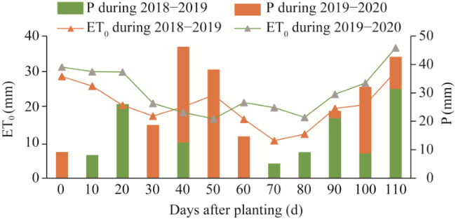
Fig. 2 Reference evapotranspiration (ET0) and precipitation (P) in wheat-growing season during the two years

2.3 Data analysis

The calibration of the AquaCrop model utilized meteorological data and measured plant and field data collected during the first year to simulate yield changes at different irrigation timings. To validate the simulated results, we implemented the most suitable scenario suggested by the model in the second year on the selected farms, and compared and evaluated the obtained results against the model's simulation. Measurements indicated that the maximum depth of wheat roots was approximately 40 cm. Considering the root depth and the soil's physical characteristics in the area, we used the Equation 2 to calculate the net water requirement (dn).
d n = i = 1 n F C i P W P i 100 × D i,
where dn is the net irrigation need (mm); FCi is the field capacity of the soil layer i (%); PWPi is the permanent wilting point of the soil layer i (%); Di is the thickness of the soil layer i (mm); and n is the number of soil layers.
In the three selected farms, soil permeability was measured in three repetitions (totalling nine measurements) using a double-ring infiltrometer under field conditions during plant establishment. Based on the average measurements, we calculated the infiltration by Equation 3:
F = 14.04 t 0.15 + 4 t,
where F is the cumulative infiltration (mm); and t is the duration of contact between water and soil (h).
Using this equation, we defined infiltration conditions for the WinSRFR model according to the recommendations of Strelkoff and Clemmens (2007), employing the modified Kostiakov-Lewis method. Average final infiltration rate in the plots was 4 mm/h. The heavy soil texture and high bulk density (1.51 g/cm3) contributed to a decrease in the rate of water infiltration into the soil and reduced cumulative infiltration. The progression of water in the target farms is presented in Figure 3. Irrigation management information including the number of irrigation events, irrigation dates, and duration of irrigation was also determined.
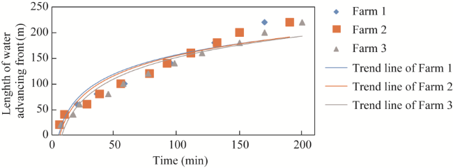
Fig. 3 Changes in the length of water advancing front in the soil of the three farms
The WinSRFR model was used to calibrate current conditions. Key parameters—such as the length, width, and discharge of irrigation borders in the study area—were determined. The flow rate of the strip was determined using the diameters of the sluice gate (''D'' in Fig. 1) in the field and the water velocity at the inlets of the gate. In addition, water flow was measured at each farm. Subsequently, the most appropriate, applicable, and practical scenario in terms of length, width, discharge, and irrigation duration for enhancing water use efficiency was identified and evaluated during the second year. Figure 4 illustrates the process of combining the results of the AquaCrop and WinSRFR models to optimize on-site water management.
As can be seen in the Figure 4, the input parameters of the Aquacrop model include weather, crop, management, and soil properties that simulate irrigation scheduling, yield, and WP, and the input parameters of the WinSRFR model include soil hydraulic properties and irrigation systems that calibrate field conditions. Finally, the results of these two models are combined and analyzed in three dimensions. Based on the indicators considered, we proposed the most appropriate method to improve water management on the farm.
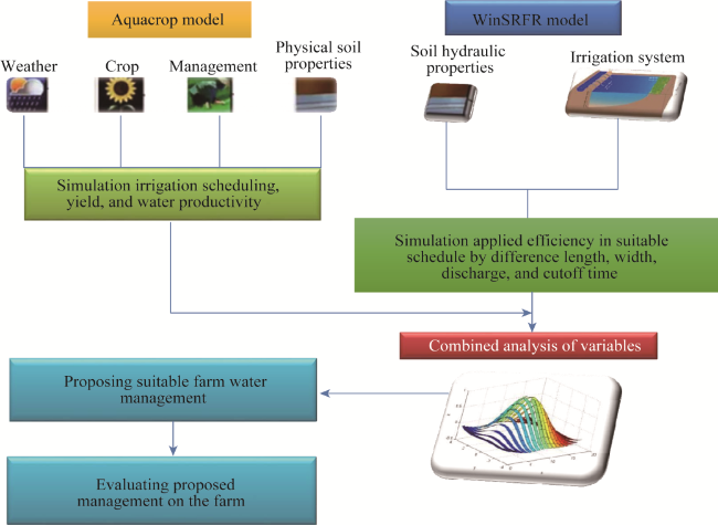
Fig. 4 Process of combining the results of the AquaCrop and WinSRFR models for farm water management

3 Results

Agricultural and plant data measured from the farms were used to calibrate the AquaCrop model. Using these measured data, simulations were performed under different irrigation schedule conditions. Various management scenarios were applied in terms of irrigation frequency to compare changes in wheat grain yield by considering different numbers of irrigation events, ranging from 3 to 6 (Table 2), which are conventional in the study area. The results demonstrate the relationship between irrigation frequency (3-6 irrigation events), grain yield, water consumption, and wheat water use efficiency in the specified trials (Table 2). Notably, there was no significant difference in grain yield and total yield between 4 and 5 irrigation events. The considered irrigation schedules followed the region's standard practices for the stages of planting, tillering, stem formation, flowering, and grain filling (totalling 5 irrigation events). Four irrigation events were allocated up to the tillering stage, while 3 irrigation events excluded the tillering and stem formation stages. The results indicated that the average total yield and wheat grain yield simulated under 4 and 5 irrigation events did not differ significantly. However, the volume of water consumed in 4 irrigation events decreased by 20.0% compared with 5 irrigation events. Consequently, the applied water use efficiency increased by 21.0% in 4 irrigation events compared with 5 irrigation events (Table 2).
Table 2 Variation of simulated wheat yield with irrigation events using the Aquacrop model
Index Farm 1 Farm 2 Farm 3
3 4 5 6 3 4 5 6 3 4 5 6
Consumed water (kg/m3) 5800 7600 9400 11,200 5800 7600 9400 11,200 5800 7600 9400 11,200
ET (mm) 234 258 270 297 272 309 323 333 267 302 329 328
Total yield (t/hm2) 4.7 5.8 5.8 6.0 6.2 7.2 7.2 7.2 5.6 6.6 6.7 6.6
Grain yield (t/hm2) 1.9 2.4 2.4 2.5 2.5 2.9 2.9 2.9 2.2 2.6 2.6 2.6
WP (kg/m3) 0.33 0.31 0.26 0.22 0.43 0.38 0.31 0.26 0.38 0.34 0.28 0.23

Note: 3-6 mean the irrigation events; ET, evapotranspiration; WP, water productivity.

Furthermore, the simulation showed that increasing irrigation during the ripening stage (April) did not significantly enhance the grain and total yield but reduced water use efficiency due to the additional irrigation event. Conversely, with only 3 irrigation events, grain yield decreased by 15.0%. Given the significant yield reduction with 3 irrigation events compared with more frequent irrigation, this scenario was not recommended for optimal performance. Therefore, based on the simulation, it was recommended to apply at least 4 irrigation events during the planting, stem elongation, flowering, and seed-filling stages to maintain an appropriate production level under existing conditions.
To validate the results obtained from the AquaCrop model in simulating wheat grain yield, we measured water consumption and yield data from the three selected farms in the second year based on the 4 irrigation events recommended from the first year's results. The climatic conditions of the second year were examined and evaluated using the model's results. The simulated wheat grain yield under normal regional conditions (5 irrigation events) averaged 2.7 t/hm2, which was not significantly different from the measured yield of 3.0 t/hm2 (Fig. 5). This similar agreement indicated that the simulated wheat yields obtained from the model aligned well with the measured values and could be reliably used to simulate different irrigation scenarios.
Fig. 5 Comparison between simulated and measured grain yields by the AquaCrop model. NRMSE, normalized root mean square error.
In each selected plot, wheat was harvested in three replicates from 1 m² areas during the first week of May. The average wheat grain yield in the second year was approximately 4400 kg/hm2. Figure 5 presents the simulated performance results in the second year using the AquaCrop model.
As shown in Figure 5, the coefficient of regression, normalized root mean square error, and agreement index were 0.924, 0.14, and 0.89, respectively. These criteria indicated the model's effectiveness and efficiency in simulating wheat yield over two consecutive years. Both the measured and simulated yields in the first year were lower than those in the second year. The key factor influencing yield differences between the two years was the timing and frequency of irrigation, which increased wheat yield in the second year, highlighting the AquaCrop model's effectiveness.
Irrigation efficiency was assessed using the WinSRFR model to determine the optimal number of irrigation events. Based on changes in the input flow rate and depth of irrigation water, Table 3 presents the range of water application efficiency. The water application efficiency in the selected plots ranged from 27.0% to 32.0%, indicating that a significant portion of water applied in the field was lost through deep percolation beyond the root zone (40 cm). The WinSRFR model, calibrated with an error range of 6.9%-10.7% (average error of 8.8%), provided a suitable estimate of efficiency under current conditions, enabling the simulation of efficiency changes with alterations in inlet flow dimensions and rates (Table 3).
Table 3 Comparison between measured and simulated application efficiencies in the first year
Farm Irrigation Stage Discharge (L/s) Water depth (mm) Net water depth (mm) Measured application efficiency (%) Simulated application efficiency (%) Standard error (%)
1 1 Initial 19 161 50 31.0 28.0 6.9
2 Development 17 185 50 27.0 25.0 7.4
3 Mid-growth 20 172 50 29.0 26.0 10.3
2 1 Initial 18 156 50 32.0 30.0 6.2
2 Development 17 160 50 31.0 28.0 9.6
3 Mid-growth 19 188 50 26.0 24.0 7.6
3 1 Initial 18 180 50 28.0 25.0 10.7
2 Development 19 165 50 30.0 27.0 10.0
3 Mid-growth 19 160 50 31.0 28.0 9.6
The results obtained for a slope of 0.2% are shown in Figure 6. The border width was set at 8 m (Fig. 6a), the minimum width necessary for a combine harvester to enter the field. The inflow to the border ranged from 15 to 22 L/s. The findings indicated that a border length between 180 and 200 m provided higher application efficiency compared with other conditions. Furthermore, the water application efficiency along a border of 180 m length and 8 m width (Fig. 6a), with a flow rate of 15-18 L/s at a slope of 0.2% and an average irrigation duration of 3.0-3.5 h, ranged from 34.0% to 38.0%. Conversely, with a border length of 200 m and the same width, if the inflow remained between 15 and 18 L/s, the average water use efficiency was approximately 34.0%.
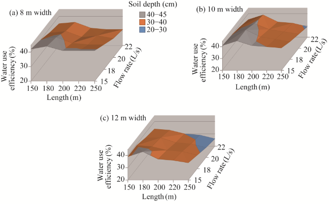
Fig. 6 WinSRFR simulation result under different border widths with a 0.2% slope. (a), 8 m width; (b), 10 m width; (c), 12 m width.
In Figure 6b, values for different lengths from 150 to 250 m, with a fixed width of 10 m and flow rates ranging from 15 to 22 L/s (slope of 0.2% and net irrigation depth of 50 mm), were evaluated and compared. The WinSRFR model results showed that when the border length and width were 180 and 10 m (Fig. 6b), respectively, and the inflow ranged from 15 to 18 L/s, and the average water use efficiency was about 43.0%. Under these conditions, the highest water use efficiency was achieved (approximately 46.0%) with an irrigation time of about 3.0-3.5 h. Notably, when the border length increased to 200 m under the same condition, the average water application efficiency at a flow rate of 15-18 L/s decreased to 41.0%.
Additionally, other lengths from 150 to 250 m with a fixed width of 12 m (Fig. 6c) and inflow rates ranging from 15 to 22 L/s (slope of 0.2% and net irrigation depth of 50 mm) were studied. Implementation of the WinSRFR model revealed that the water use efficiency was 44.0% when the border length and width were 180 and 12 m, respectively, with an inflow rate ranging from 15 to 18 L/s. If the border length increased to 200 m (width of 12 m) and irrigation duration increased, the average water use efficiency decreased to 41.0%.
For a more definitive conclusion, the highest application efficiency was obtained at a border length of 180 m. Therefore, Figure 7 illustrates the average changes in water use efficiency for the three border widths examined. The results indicated that under existing conditions, a width of 10 m was optimal. A flow rate of 15-18 L/s did not significantly decrease water use efficiency at widths of 10 and 12 m. However, at a width of 8 m, there was a greater decrease in water use efficiency due to flow rate changes. Thus, a flow rate of 15 L/s is recommended for this width. Moreover, a significant decrease in water use efficiency was observed across all three widths at a flow rate of 19 L/s, so inflows exceeding 19 L/s were not advisable for each border. While flow rates of 20-25 L/s could be applied to a border length of 180 m and a slope of 0.2% with a width of 10 m, lower discharge rate was recommended to enhance efficiency.
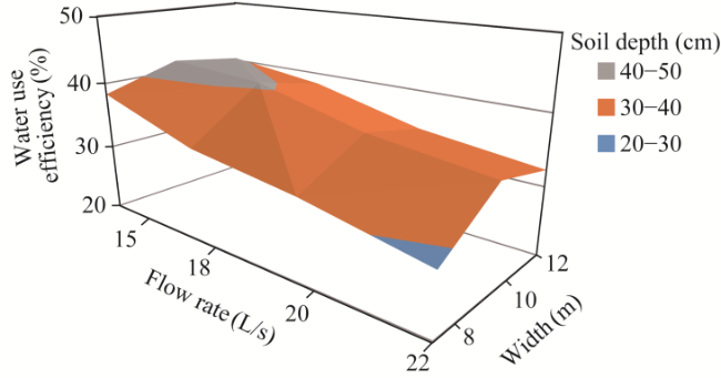
Fig. 7 Water use efficiency under different widths and discharges with a border length of 180 m
Using the results from the first year, we prepared three experimental farms in the second year based on the recommendation of the WinSRFR model. Each farm had a border length of 180 m and a width of 10 m. All parameters measured in the second year were also examined, and the results are presented in Table 4.
Table 4 Range of water productivity (WP) measured in the second year
Farm Replication Stage Flow (L/s) Depth of water (mm) Net depth of water (mm) Measured water application efficiency (%) Simulated water application efficiency (%) Standard error
(%)
WP (kg/m3)
Farm 1 1 Initial 18 110 50 45.0 40.0 11.0 0.97
2 Development 20 115 50 43.0 37.0 14.0 0.81
3 Mid-growth 22 120 50 41.0 35.0 15.0 0.97
Farm 2 1 Initial 18 114 50 44.0 40.0 9.0 1.01
2 Development 20 142 50 35.0 37.0 6.0 0.80
3 Mid-growth 22 152 50 33.0 35.0 6.0 0.75
Farm 3 1 Initial 18 108 50 46.0 40.0 13.0 0.98
2 Development 20 125 50 40.0 37.0 8.0 0.89
3 Mid-growth 22 132 50 38.0 35.0 8.0 0.83
Average 1 Initial 18 111 50 45.0 40.0 11.0 0.99
2 Development 20 127 50 39.0 37.0 9.0 0.83
3 Mid-growth 22 135 50 37.0 35.0 10.0 0.85
Table 4 indicated that in the second year, the model accurately estimated border irrigation conditions, with errors ranging from 6.0% to 15.0%. A flow rate of 18 L/s achieved the highest water application efficiency, highlighting the WinSRFR model's effectiveness in recommending this flow rate. By implementing the management strategies suggested by both the AquaCrop and WinSRFR models, the average water consumption efficiency increased from 0.3 kg/m³ under farmers' current practices to 0.99 kg/m³ in the second year. Therefore, adjusting irrigation schedules, dimensions, and flow rates using the WinSRFR and AquaCrop models can significantly improve water use efficiency, promoting proper irrigation management on farms.

4 Discussion

Water use efficiency is extremely low in the agriculture of Iran, and many water management schemes perform poorly. This study proposed a method for identifying various factors influencing water management and provided strategies to address current issues in the irrigation. The AquaCrop and WinSRFR models are highly beneficial and can be applied in irrigation management (Abi Saab et al., 2015; Xu et al., 2019; Mazarei et al., 2020; Corbari et al., 2021). The findings demonstrate the effectiveness of the AquaCrop model in simulating wheat yield over two consecutive years (Fig. 5). Irrigation timing is a major factor affecting yield variations between different years. In this case, the AquaCrop model performed well, as evidenced by the increased wheat yield in the second year. Corbari et al. (2021) improved water use efficiency for maize and tomato in Italy using the AquaCrop model. The model is based on an operational optimization irrigation strategy that considers crop stress thresholds and evaluates the impact of irrigation volumes and frequency on crop yield, canopy cover, and the main source of water loss—water is not used by the plants and lost through cumulative drainage flux. The AquaCrop model was validated and the mean absolute errors of ET, maize yield, and tomato yield were 0.3-0.9 mm/d, 0.9 t/hm2, and 10.0 t/hm2, respectively.
Improved water and soil management in the field can explain differences between actual and potential yields. Simulations of the AquaCrop model on crop water requirements aligned with satellite remote sensing estimations. For maize, actual satellite remote sensing estimates in the Kou Valley (southwestern Burkina Faso) were 549 mm/season, while the study reported 387 mm/season under net irrigation requirements (Sawadogo et al., 2020). However, standalone program of the AquaCrop model has the drawback of being time-consuming when assessing crop water requirements. To overcome this, researcher developed a semi-automated software environment to run and evaluate field-level simulation simultaneously (Sallah et al., 2019). The AquaCrop model assumes uniform fields without spatial differences in crop development, transpiration, soil characteristics, or management, considering only vertical incoming and outgoing fluxes and overlooking horizontal water movement. However, developing an irrigation decision support system is complex and requires collaboration between national institutions and farmers. One solution is to create a dashboard for user-friendly irrigation programming and monitoring consultation (Ferrández-Pastor et al., 2018).
A review of earlier studies indicates that irrigation duration, inflow rate, and strip length and width are among the most significant factors influencing water use efficiency (Tafteh and Emdad, 2017; Radmanesh et al., 2023; Zahedpour Yeganeh et al., 2024). The findings demonstrate that the WinSRFR model, with an average error of 9.0%, provides a reasonable estimate of efficiency under current conditions and can be used to simulate applied efficiency when the inlet flow's dimension and flow rate change (Table 2). Radmanesh et al. (2023) studied irrigation performance in continuous and surge irrigation by furrows using the WinSRFR and SIRMOD models. They found that these models are reliable for evaluating furrow irrigation strategies and improving management. The study suggests that irrigation engineers can use surface irrigation models to design optimized furrow lengths and stream sizes in arid and semi-arid areas for efficient water management.
Researchers implemented the WinSRFR model under various conditions based on initial information such as border dimension, inlet flow, irrigation duration, slope, and infiltration data, all crucial for surface irrigation (Navabian et al., 2009). Various parameters appropriate and applicable to the regional conditions were considered, including different lengths (150-250 m), widths (8-12 m), flow rates (15-22 L/s), and irrigation durations, to assess their impacts on efficiency. This multivariate approach is recommended for effective surface irrigation management and water use efficiency (Sanchez et al., 2009; Ma et al., 2010). The average water use efficiency achieved at a border length of 180 m, width of 10 m, flow rate of 15-18 L/s, and irrigation duration of 3.5-4.0 h was approximately 46.0%. This result is consistent with findings reported by Raghuwanshi et al. (2011) and Abbasi and Sheini Dashtegol (2017), who reported higher irrigation efficiencies of approximately 43.0%-50.0%.
The results of the second-year evaluation (Table 3) revealed that both the AquaCrop and WinSRFR models accurately estimated border irrigation conditions. A flow rate of 18 L/s was found to achieve the highest water efficiency. By utilizing a combination of these models, farmers were able to increase their average water consumption efficiency from 0.30 to 0.99 kg/m³ in the second year. Effective management of irrigation schedules, dimensions, and flow rates is crucial for improving water use efficiency. These findings align with those of previous studies by Alavi et al. (2022) and Khoshsirat et al. (2022). The results obtained from the AquaCrop and WinSRFR models are within a reasonable range and consistent with international recommendations (Alavi et al., 2022). However, the precise amount of infiltration is crucial and can only be accurately determined through modelling and direct measurement; otherwise, recommendations remain general. Surface irrigation is optimized and simulated using the WinSRFR model, which also helps determine the best furrow length, flow rate, and other parameters for surface irrigation to maximize water use in the field. The AquaCrop model is used together with irrigation management optimization and scenario selection after the WinSRFR model has optimized furrow length and flow per unit width. Therefore, the combination of these two models will improve water use efficiency and increase productivity. These two models can therefore be utilized in other arid farms by utilizing the basic information about the soil, water, plant, and climate. The findings of this research are applicable to the specific infiltration levels and existing conditions of the study area. Therefore, it is recommended that irrigation methods could be evaluated and optimized using the AquaCrop and WinSRFR models in similar farms.

5 Conclusions

Given that changes in climatic condition, especially precipitation, significantly affect plant performance, it is recommended to predict and simulate crop performance under different water and soil conditions using the AquaCrop model. Additionally, adjusting the length of existing borders from 200 to 180 m using the WinSRFR model increased water use efficiency to 46.0% in the second year. Therefore, to enhance water use efficiency in the Hamidiyeh farms, it is suggested to set the border length to 180 m, width to 10 m, flow rate to 15-18 L/s, and irrigation duration to 3.0-3.5 h in the irrigation to achieve approximately 46.0% field water use efficiency. The combined use of the AquaCrop and WinSRFR models provides comprehensive management solutions for farmers in the study area. This approach has proven highly effective in increasing water use efficiency and achieving the overarching goals of irrigation management in the Khuzestan Province, Iran. Fortunately, the application of these models is not restricted to any particular area. Therefore, they can be used in any climate by providing basic information such as soil, water, plant, and climate.

Conflict of interest

The authors declare that they have no known competing financial interests or personal relationships that could have appeared to influence the work reported in this paper.

Acknowledgment

The study was funded by the Soil and Water Research Institute of Iran. We appreciated the help of the Agricultural Research, Education, and Extension Organization, Iran.

Author contributions

Conceptualization: Arash TAFTEH, Mohammad R EMDAD, Azadeh SEDAGAT; Data curation: Arash TAFTEH, Mohammad R EMDAD; Formal analysis: Arash TAFTEH, Mohammad R EMDAD, Azadeh SEDAGAT; Investigation: Arash TAFTEH, Mohammad R EMDAD, Azadeh SEDAGAT; Methodology: Arash TAFTEH, Mohammad R EMDAD; Project administration: Arash TAFTEH, Mohammad R EMDAD; Resources: Arash TAFTEH, Mohammad R EMDAD; Software: Arash TAFTEH, Mohammad R EMDAD; Validation: Arash TAFTEH, Mohammad R EMDAD, Azadeh SEDAGAT; Writing - original draft preparation: Arash TAFTEH, Mohammad R EMDAD, Azadeh SEDAGAT; Writing - review and editing: Arash TAFTEH, Mohammad R EMDAD, Azadeh SEDAGAT; Visualization: Arash TAFTEH, Mohammad R EMDAD, Azadeh SEDAGAT; Supervision: Mohammad R EMDAD. All authors approved the manuscript.
[1]
Abbasi F, Sheini Dashtegol A. 2017. Evaluating and improving the sugarcane furrow irrigation management in Khuzestan. Water and Soil Science, 26(4): 109-121.

[2]
Abi Saab M T, Todorovic M, Albrizio R. 2015. Comparing AquaCrop and CropSyst models in simulating barley growth and yield under different water and nitrogen regimes. Does calibration year influence the performance of crop growth models? Agricultural Water Management, 147: 21-33.

[3]
Afshar A, Neshat A. 2013. Evaluation of AquaCrop computer model in the potato under irrigation management of continuity plan of Jiroft region, Kerman, Iran. International Journal of Advanced Biological and Biomedical Research, 1(2): 1669-1678.

[4]
Alavi S A, Naseri A A, Ritzema H, et al. 2022. A combined model approach to optimize surface irrigation practice: SWAP and WinSRFR. Agricultural Water Management, 271: 107741, doi: 10.1016/j.agwat.2022.107741.

[5]
Amirouche M, Smadhi D, Zella L. 2021. Calibration and validation of the AquaCrop model for the culture lettuce (Lactuca sativa L.) under fertilization levels in pluvial condition. Agricultural Engineering International: CIGR Journal, 23(1): 36-44.

[6]
Asana R, Kale V. 1965. A study of salt tolerance of four varieties of wheat. Indian Journal of Plant Physiology, 8: 5-22.

[7]
Chen B, Ouyang Z, Sun Z G, et al. 2013. Evaluation on the potential of improving border irrigation performance through border dimensions optimization: A case study on the irrigation districts along the lower Yellow River. Irrigation Science, 31: 715-728.

[8]
Corbari C, Ben Charfi I, Mancini M. 2021. Optimizing irrigation water use efficiency for tomato and maize fields across Italy combining remote sensing data and the aquacrop model. Hydrology, 8(1): 39, doi: 10.3390/hydrology8010039.

[9]
Ferrández-Pastor F J, García-Chamizo J M, Nieto-Hidalgo M, et al. 2018. Precision agriculture design method using a distributed computing architecture on internet of things context. Sensors, 18(6): 1731, doi: 10.3390/s18061731.

[10]
Forouzani M, Karami E. 2011. Agricultural water poverty index and sustainability. Agronomy for Sustainable Development, 31: 415-431.

[11]
Guendouz A, Hafsi M, Moumeni L, et al. 2014. Performance evaluation of aquacrop model for durum wheat (Triticum durum Desf.) crop in semi arid conditions in Eastern Algeria. International Journal of Current Micriobology and Applied Science, 3(2): 168-176.

[12]
Hjorth P, Madani K. 2014. Sustainability monitoring and assessment: new challenges require new thinking. Journal of Water Resources Planing and Management, 140(2): 133-135.

[13]
Horne A C, O'Donnell E L, Loch A J, et al. 2018. Environmental water efficiency: Maximizing benefits and minimizing costs of environmental water use and management. Wiley Interdisciplinary Reviews: Water, 5(4): e1285, doi: 10.1002/wat2.1285.

[14]
Keshavarz M, Karami E, Vanclay F. 2013. The social experience of drought in rural Iran. Land Use Policy, 30(1): 120-129.

[15]
Khoshsirat A M, Najarchi M, Jafarinia R, et al. 2022. Sensitivity analysis and determination of the optimal level of water use efficiency for winter wheat and barley under different irrigation scenarios using the AquaCrop Model in arid and semiarid climatic conditions (Case Study: Dehloran Plain, Iran). Water, 14(21): 3455, doi: 10.3390/w14213455.

[16]
Kumar P, Sarangi A, Singh D, et al. 2014. Evaluation of AquaCrop model in predicting wheat yield and water productivity under irrigated saline regimes. Irrigation and Drainage, 63(4): 474-487.

[17]
Ma J J, Sun X H, Guo X H, et al. 2010. Multi-objective fuzzy optimization model for border irrigation technical parameters. Journal of Drainage and Irrigation Machinery Engineering, 28(2): 160-163, 178. (in Chinese)

[18]
Madani K. 2014. Water management in Iran: what is causing the looming crisis? Journal of Environmental Studies and Sciences, 4: 315-328.

[19]
Mazarei R, Mohammadi A S, Naseri A A, et al. 2020. Optimization of furrow irrigation performance of sugarcane fields based on inflow and geometric parameters using WinSRFR in Southwest of Iran. Agricultural Water Management, 228: 105899, doi: 10.1016/j.agwat.2019.105899.

[20]
Navabian M, Liaghat A, Smith R, et al. 2009. Empirical functions for dependent variables in cutback furrow irrigation. Irrigation Science, 27: 215-222.

[21]
Nazari B, Liaghat A, Akbari M R, et al. 2018. Irrigation water management in Iran: Implications for water use efficiency improvement. Agricultural Water Management, 208: 7-18.

[22]
Nie W B, Fei L J, Ma X Y. 2014. Applied closed-end furrow irrigation optimized design based on field and simulated advance data. Journal of Agricultural Science and Technology, 16(2): 395-408.

[23]
Radmanesh M, Ahmadi S H, Sepaskhah A R. 2023. Measurement and simulation of irrigation performance in continuous and surge furrow irrigation using WinSRFR and SIRMOD models. Scientific Reports, 13: 5768, doi: 10.1038/s41598-023-32842-8.

[24]
Raes D, Steduto P, Hsiao T C, et al. 2009. AquaCrop—the FAO crop model to simulate yield response to water: II. main algorithms and software description Agronomy Journal, 101(3): 438-447.

[25]
Raghuwanshi N, Damodhara R, Mailapalli S, et al. 2011. Infiltration evaluation strategy for border irrigation management. Journal of Irrigation and Drainage Engineering, 137(9): 601-609.

[26]
Sallah A H M, Tychon B, Piccard I, et al. 2019. Batch-processing of AquaCrop plug-in for rainfed maize using satellite derived Fractional Vegetation Cover data. Agricultural Water Management, 217: 346-355.

[27]
Sanchez C, Zerihun D, Farrell-Poe K. 2009. Management guidelines for efficient irrigation of vegetables using closed-end level furrows. Agricultural Water Management, 96(1): 43-52.

[28]
Sawadogo A, Kouadio L, Traoré F, et al. 2020. Spatiotemporal assessment of irrigation performance of the Kou Valley irrigation scheme in Burkina Faso using satellite remote sensing-derived indicators. ISPRS International Journal of Geo-Information, 9(8): 484, doi: 410.3390/ijgi9080484.

[29]
Strelkoff T S, Clemmens A J. 2007. Hydraulics of Surface Systems, Design and Operation of Farm Irrigation Systems (2nd ed.). St. Joseph: American Society of Agricultural and Biological Engineers, 436-498.

[30]
Tafteh A, Emdad M R. 2017. Improvement of water use productivity through the SRFR model in border strip irrigation of wheat across Hamidiyeh farms (Khuzestan, Iran). Fresenius Environmental Bulletin, 25(12): 7885-7892.

[31]
Taghizadeh Z, Verdinejad V R, Ebrahimian H, et al. 2013. Field evaluation and analysis of surface irrigation system with WinSRFR (case study furrow irrigation). Water and Soil, 26(6): 1450-1459.

[32]
Thebuwena A C H J, Samarakoon S S M, Ratnayake R C. 2024. On the necessity for improving water efficiency in commercial buildings: A green design approach in hot humid climates. Water, 16(17): 2396, doi: 10.3390/w16172396.

[33]
Wale A, Dessie M, Kendie H. 2022. Evaluating the performance of AquaCrop model for potato production under deficit irrigation. Air, Soil and Water Research, 15(1): 1-14.

[34]
Xu J T, Cai H J, Saddique Q, et al. 2019. Evaluation and optimization of border irrigation in different irrigation seasons based on temporal variation of infiltration and roughness. Agricultural Water Management, 214: 64-77.

[35]
Zahedpour Yeganeh H, Khorsand A, Rezaverdinejad V, et al. 2024. Field assessment and analysis of border irrigation systems with WinSRFR software (case study: Urmia Plain wheat fields). Water and Soil Management and Modeling, 4(3): 187-202.

[36]
Zhai Y, Huang M, Zhu C, et al. 2022. Evaluation and application of the AquaCrop model in simulating soil salinity and winter wheat yield under saline water irrigation. Agronomy, 12(10): 2313, doi: 10.3390/agronomy12102313.

[37]
Zhang W H, Liu W Z, Xue Q W, et al. 2013. Evaluation of the AquaCrop model for simulating yield response of winter wheat to water on the southern Loess Plateau of China. Water Science and Technology, 68(4): 821-828.

[38]
Zhou Q, Zhang Y L, Wu F. 2021. Evaluation of the most proper management scale on water use efficiency and water productivity: A case study of the Heihe River Basin, China. Agricultural Water Management, 246: 106671, doi: 10.1016/j.agwat.2020.106671.

文章导航

/