• MIAO Jiamin 1, 2, 3 ,
  • LI Shengyu , 1, 2, 3, * ,
  • XU Xinwen 1, 2, 3 ,
  • LIU Guojun 1, 2, 3 ,
  • WANG Haifeng 1, 2, 3 ,
  • FAN Jinglong 1, 2, 3 ,
  • Khaulanbek AKHMADI 4
展开

收稿日期: 2024-05-19

  修回日期: 2024-07-17

  录用日期: 2024-07-23

  网络出版日期: 2025-08-12

Benefits and ecological restoration implications of hanging grass fences in Mongolian desert steppe

  • MIAO Jiamin 1, 2, 3 ,
  • LI Shengyu , 1, 2, 3, * ,
  • XU Xinwen 1, 2, 3 ,
  • LIU Guojun 1, 2, 3 ,
  • WANG Haifeng 1, 2, 3 ,
  • FAN Jinglong 1, 2, 3 ,
  • Khaulanbek AKHMADI 4
Expand
  • 1Key Laboratory of Ecological Safety and Sustainable Development in Arid Lands, Xinjiang Institute of Ecology and Geography, Chinese Academy of Sciences, Urumqi 830011, China
  • 2National Engineering Technology Research Center for Desert-Oasis Ecological Construction, Xinjiang Institute of Ecology and Geography, Chinese Academy of Sciences, Urumqi 830011, China
  • 3University of Chinese Academy of Sciences, Beijing 100049, China
  • 4Institute of Geography and Geoecology, Mongolian Academy of Sciences, Ulaanbaatar 15170, Mongolia
*LI Shengyu (E-mail: )

Received date: 2024-05-19

  Revised date: 2024-07-17

  Accepted date: 2024-07-23

  Online published: 2025-08-12

本文引用格式

MIAO Jiamin , LI Shengyu , XU Xinwen , LIU Guojun , WANG Haifeng , FAN Jinglong , Khaulanbek AKHMADI . [J]. Journal of Arid Land, 2024 , 16(11) : 1541 -1561 . DOI: 10.1007/s40333-024-0063-6

Abstract

Tumbleweeds participate in a common seasonal biological process in temperate grasslands, creating hanging grass fences during the grass-withering season that result in distinct ecological phenomena. In this study, we addressed the urgent need to understand and restore the degraded desert steppe in Central Mongolia, particularly considering the observed vegetation edge effects around hanging grass fences. Using field surveys conducted in 2019 and 2021 in the severely degraded desert steppe of Central Mongolia, we assessed vegetation parameters and soil physical and chemical properties influenced by hanging grass fences and identified the key environmental factors affecting vegetation changes. The results indicate that the edge effects of hanging grass fences led to changes in species distributions, resulting in significant differences in species composition between the desert steppe's interior and edge areas. Vegetation parameters and soil physical and chemical properties exhibited nonlinear responses to the edge effects of hanging grass fences, with changes in vegetation coverage, aboveground biomass, and soil sand content peaking at 26.5, 16.5, and 6.5 m on the leeward side of hanging grass fences, respectively. In the absence of sand dune formation, the accumulation of soil organic carbon and available potassium were identified as crucial factors driving species composition and increasing vegetation coverage. Changes in species composition and plant density were primarily influenced by soil sand content, electrical conductivity, and sand accumulation thickness. These findings suggest that hanging grass fences have the potential to alter vegetation habitats, promote vegetation growth, and control soil erosion in the degraded desert steppe of Central Mongolia. Therefore, in the degraded desert steppe, the restoration potential of hanging grass fences during the enclosure process should be fully considered.

1 Introduction

Grasslands face an ongoing and severe threat of continuous degradation, weakening their ability to sustain biodiversity, regulate climate, sequester carbon, and provide livestock fodder (Allan et al., 2015; Eldridge and Delgado-Baquerizo, 2017; Bai and Cotrufo, 2022; Yan et al., 2023). Situated in arid and semi-arid areas, the grasslands in Mongolia are one of the most climate-sensitive regions worldwide (Seddon et al., 2016). Severe and frequent droughts combined with overgrazing impede vegetation recovery after disturbances, exacerbating grassland degradation and intensifying desertification (Zhang et al., 2020; Sainnemekh et al., 2022). About 77.8% of the total area in Mongolia has experienced increasing degradation to varying degrees (Khaulanbek et al., 2013). Grassland degradation has also led to frequent and substantial environmental problems, further resulting in warnings being issued about the ecological security of neighbouring countries and regions, such as dust storms (Hu et al., 2023).
Fencing enclosures are widely used to reduce grazing pressure in grasslands because of their cost-effectiveness, immediate effect, and ease of implementation (Hao et al., 2021; Zheng et al., 2023). Fencing facilities divide grasslands into several parts, allowing enclosed areas to gradually experience self-restoration once human and livestock disturbances have been eliminated (Liu et al., 2023). After fencing facilities are established, vegetation coverage, plant height, plant biomass, and the proportion of high-quality forage in enclosed areas are significantly higher than those in grazed areas (Sanaei et al., 2019; Du et al., 2020; Ju et al., 2023). Grazing exclusion aids in controlling soil erosion and promotes surface litter accumulation and nutrient input from root turnover into the soil, which effectively enhances the nutrients and physical and chemical properties of the soil (Wang et al., 2021; Xu et al., 2023). Most prior studies assessing the impact of fencing enclosures have primarily concentrated on comparative analyses that treat the interior and exterior of fences as unified entities (Xiong et al., 2016; Sainnemekh et al., 2022; Liu et al., 2023). The necessity of sampling at least 10 m away from the fences to avoid edge effects has also been emphasised (Feyisa et al., 2017; Zhang et al., 2019). The fenced areas in grasslands create multiple patches within the grassland matrix. Edge effects of enclosure facilities often occur at the edges between fenced patches and the surrounding grassland matrix (Hamm and Drossel, 2017). The extent and magnitude of the edge effects of enclosure facilities may be largely influenced by their structural features. This is because edge effects are highly sensitive to contextual factors such as edge orientation and edge contrast (Porensky, 2011). To date, relatively little research has been conducted on the impact of edge effects on the efficacy of fenced areas.
Enclosure facilities comprise mechanical fences made of materials such as wire or iron mesh and biological fences formed by linearly planted trees or shrubs as an enclosure (Wang et al., 2021; Munoz-Cerro et al., 2023). Nevertheless, tumbleweeds are important in species dispersal during the grass-withering season in grasslands. This is because their main stems break off close to the ground and roll with the wind (Becker, 1978; Baker and Beck, 2008). During their spread, tumbleweeds could be intercepted by fencing facilities, accumulating or hanging on these facilities, forming the biological-mechanical fences known as 'hanging grass fences'. However, it remains unknown whether this distinctive ecological phenomenon influences the efficacy of grassland enclosures. The edge areas adjacent to linear barriers like biological fences differ significantly from the surrounding core habitats (Haddaway et al., 2018; Schopke et al., 2023). Ecological edge effects can significantly alter species composition and richness in the edge areas (Hamm and Drossel, 2017). For instance, hedges, acting as biological corridors that connect separated habitats, can provide favourable habitats for generalist species, leading to greater species richness (Liira and Paal, 2013). Changes in species composition are primarily caused by the increased presence of alien species and their adaptability to edge environments (Boutin et al., 2008; Schopke et al., 2023). Edge effects manifest in creating gradients in soil physical and chemical properties and microclimates from the edge to the interior (Gasperini et al., 2021; Novaes et al., 2022). Zheng et al. (2016) found that shelterbelts effectively reduced the wind speed on the leeward side, with this wind moderation effect extending up to 20 times the tree height. Reduced wind speeds may decrease soil moisture evaporation (Vacek et al., 2018; Veste et al., 2020). In the forest-grassland mosaic, edge effects lead to increased soil temperature and decreased soil moisture content, nutrient cycling efficiency, and litter decomposition rates (Burst et al., 2020; Cardelús et al., 2020). However, Wang et al. (2021) found that when edges separated similar habitat types, edge effects from fencing facilities could lead to significant variations in plant biomass and soil organic carbon (SOC) content. There were higher plant biomass and SOC content values closer to the fences, despite the relatively small contrast between the inside and outside of the fenced areas. However, the spatial distribution of vegetation characteristics and soil physical and chemical properties within grassland enclosures featuring hanging grass fences remains poorly understood.
In practice, hanging grass fences reduce the porosity and alter the structure of the original mechanical fences. This alteration may slow the flow of matter and energy between grazed and enclosed areas (Ries and Sisk, 2004). Previously, hanging grass fences were regarded as an important measure for mitigating wind and snow damage on grassland roads because they can effectively block wind-drifting snow with a structure similar to that of wind deflectors (Kinar, 2017; Li et al., 2022; Ma et al., 2022). However, there have been few investigations on whether hanging grass fences can affect grassland enclosures during the vegetation regreening period. Therefore, in this study, we focused on the severely degraded desert steppe in Central Mongolia, aiming to quantify the ecological restoration effects (including edge effects) of hanging grass fences and explore their mechanisms. We aimed to address the following questions: (1) how do the duration of enclosure with hanging grass fences (GF) and enclosure with non-hanging grass fences (NF) and the presence of hanging grasses on fences affect vegetation and soil? (2) how do vegetation and soil respond to edge effects, especially the distance from fences in relation to different enclosure treatments? and (3) what are the key environmental factors explaining the changes in vegetation after enclosure? The findings can provide a better understanding of the role of hanging grass fences in the restoration of degraded grasslands and sustainable grassland ecosystem management in Central Mongolia.

2 Materials and methods

2.1 Study area

The study was conducted in a degraded desert steppe of Choir in Govisumber Province, Central Mongolia (45°52′-46°59′N, 107°53′-109°07′E). Figure 1 shows the sampling locations for the field surveys, climate characteristics during the sampling period, and the structure of hanging grass fences in the region. The regional climate has considerable daily and annual temperature fluctuations and irregular precipitation, belonging to a continental climate. With a mean annual temperature of 2.0°C, the monthly temperature variations range from -9.7°C (coldest in January) to 21.2°C (warmest in July). The annual precipitation averages 150.8 mm, mainly falling during the vegetation growing season, which accounts for approximately 70% of the total annual precipitation. The mean annual wind speed is 3.9 m/s. This is attributed to the flat terrain and lack of steep mountains in the region. The soils are categorised as Kastanozem, a classification based on the World Reference Base for Soil Resources system, and distinguished by texture, including loam, sandy loam, and gravelly light loam (Li et al., 2006). The dominant plant species mainly consist of Stipa krylovii and Artemisia frigida, which are interspersed with Caragana shrubs. Spring is characterised by increased windiness, rising temperatures, and sporadic late precipitation (Fig. 1c). This results in arid ground surfaces and hinders vegetation growth. Fine particles from the ground surface are easily carried away by wind erosion, which is a natural driving force for the degradation of regional grasslands (Meng et al., 2020). However, the grazing activity in this region has steadily increased, reaching a grazing intensity of 78 heads/km2 by 2021. Therefore, overgrazing has become the most impactful socioeconomic factor in the degradation of desert steppe (Yan et al., 2023).
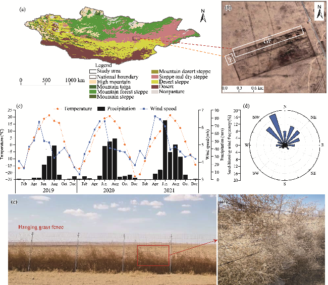
Fig. 1 Overview of the study area, climate characteristics, and hanging grass fences. (a), location of the study area (the study area is located in the ecotone of steppe and desert steppe in Central Mongolia); (b), image showing the experimental design; (c), monthly variations in temperature, precipitation, and wind speed during the sampling period (2019-2021); (d), frequency of sand-driving winds at 10 m in height with wind rose directions; (e), photo showing the hanging grass fence during the grass-withering season (April) in 2019; (f), photo showing the tumbleweeds hanging and accumulating on the fence in April 2019. Note that Figure 1a is based on the standard map (GS(2016)1666) of the Map Service System (http://bzdt.ch.mnr.gov.cn/), and the boundary of the base map has not been modified. The enclosure in Figure 1b is shown in a true-colour image downloaded from Google Earth, including enclosure with hanging grass fences (abbreviated as GF) and enclosure with non-hanging grass fences (abbreviated as NF). N, north; NE, northeast; E, east; SE, southeast; S, south; SW, southwest; W, west; NW, northwest. The abbreviations are the same in the following figures.
In the early spring of 2019, a 20.0-hm2 enclosure was established in the northern suburban grazing area (Fig. 1b), surrounded by fencing facilities (mesh size of 20.0 cm×7.0 cm) 1.8 m above the ground. During the grass-withering season, fencing effectively inhibited the spread of tumbleweeds. Subsequently, a substantial amount of tumbleweed residue hanging and accumulating on the fences perpendicular to the prevailing wind direction (northwest) formed hanging grass fences with a low density and sparse upper porosity of approximately 40% (measured in May 2019) (Fig. 1e). However, following the regreening period of the desert steppe, a distinct natural green belt emerged on the leeward side of the fences (Fig. 2). Meanwhile, the fences in other directions did not exhibit such a gradient of vegetation recovery.
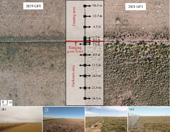
Fig. 2 Experimental design and sampling locations for vegetation and soil survey. (a), drone images showing example locations of transects and sample plots; (b), photo showing vegetation recovery during the early formation of the hanging grass fences in April 2019; (c), photo showing the regreening of the grassland in August 2019 for the first year of enclosure with hanging grass fences (GF1); (d), photo showing the regreening of the grassland in August 2021 for the third year of enclosure with hanging grass fences (GF3); (e), photo showing the third year of enclosure with non-hanging grass fences (NF3). Positive distances indicate sample plots within the enclosure area on the leeward side of the fences, and negative distances indicate sample plots within the grazing area on the windward side of the fences. The abbreviations are the same in the following figures.

2.2 Field surveys and sample collection

To quantify the gradual transition between stable vegetation states on either side of the fencing facility, we conducted field surveys and collected vegetation and soil samples in August 2019 and August 2021 using the line transect method (Michels et al., 2017). We set up transects within each of the fencing facility segments using systematic random sampling, ensuring a minimum distance of 30.0 m between segments to account for spatial variability. A mixed effect model analysis was conducted, with the duration of GF and the presence of hanging grasses on the fences as fixed effects and the transect segments of the fencing facilities as random effects to avoid pseudo-replication.
This study was initiated in 2019 and marked the first year of enclosure with hanging grass fences (abbreviated as GF1; Fig. 2c). Three transects, each extending 22.0 m, were established on the leeward side of the enclosure area. Sample plots of 1.0 m×1.0 m in size were positioned starting 1.5 m from the fences, maintaining a regular interval of 5.0 m between plots. Five sample plots were randomly selected within the grazing area on the windward side to observe the preliminary effects of hanging grass fences on grazing exclusion. In 2021, marking the third year of enclosure with hanging grass fences (abbreviated as GF3; Fig. 2d), the green belt extended beyond 22.0 m. To monitor the edge effects of hanging grass fences, we extended the transects to 44.0 m. The sample plot centres ranged from 16.5 m on the windward side of the fences to 26.5 m on the leeward side, maintaining consistent plot sizes and spacing with those in 2019. Sand accumulation occurred at the fences on the side with hanging grasses, leading us to refine the area immediately adjacent to the fences by adding plots at 0.5 m from the fence edge. The third year of enclosure with non-hanging grass fences (abbreviated as NF3; Fig. 2f), which were aligned with the direction of the prevailing wind and lacked hanging grass, was utilized as the control group to investigate the effects of hanging grass fences on edges. Nine transects, comprising 92 sample plots, were established during the sampling process.
The taxa, coverage, number of plants, and average height of each taxon were measured for each sample plot in the field. We measured aboveground biomass by clipping the aboveground parts of the plants, drying them at 65.0°C, and subsequently weighing them. We used stainless-steel augers to collect composite samples from different positions (corners and centres) within the pre-surveyed vegetation plots. In 2019, topsoil samples were collected from the depth of 0-10 cm because of the high root content of grassland plants. This layer of soil is extremely vulnerable to environmental factors and grazing demands (Bell et al., 2011). However, in 2021, soil samples were collected from the depths of 0-10 and 10-30 cm after frequent wind and sand disturbances. The collected soil samples were air-dried, passed through a 2-mm sieve to remove stones and roots, and stored at -20.0°C before being assessed through standard methods (Bao, 2000). Soil pH and electrical conductivity (EC) were measured in a 1:5 soil:water suspension using a glass electrode acidimeter (Leici PHSJ-5, INESA Scientific Instrument Co., Ltd., Shanghai, China) and an EC metre (Leici DDSJ-318, INESA Scientific Instrument Co., Ltd., Shanghai, China), respectively. Soil water content (SWC) was assessed using the oven drying method. SOC was quantified using the dichromate oxidation technique. Available phosphorus (AP) was estimated using the 0.5 mol/L NaHCO3 molybdenum antimony colorimetric method. Meanwhile, available potassium (AK) was evaluated using NH4OAC atomic absorption spectrophotometry. Particle size analysis was conducted using a laser particle-size analyzer (BT-2001, Bettersize Instruments Ltd., Dandong, China) to determine the proportions of clay (<0.002 mm), silt (0.002-0.050 mm), and sand (0.050-2.000 mm).

2.3 Statistical analysis

Before data analysis, we checked the normality, homogeneity, and overdispersion of the data. All the statistical analyses were conducted using R v.3.6.1 (R Core Team, 2023), with the significance level set at less than 5%. The ''lme4'' package was used for linear mixed model (LMM) analyses (Bates et al., 2015), and the ''car'' (Fox and Weisberg, 2019) and ''lsmeans'' (Lenth, 2016) packages were used for least-squares mean estimation and contrast tests, respectively. The ''vegan'' package (Oksanen et al., 2020) was used for nonmetric multidimensional scaling (NMDS), permutational multivariate analysis of variance (PERMANOVA), and canonical correspondence analysis (CCA). The ''lavaan'' package (Rosseel, 2012) was used for structural equation modelling (SEM) analysis.
We used the method of Luo et al. (2019) to calculate the importance values of plant species within each sample plot. During the application of the three distinct enclosure treatments (GF1, GF3, and NF3), NMDS was used to investigate the changes in the vegetation community at different distances from the fences. PERMANOVA was conducted to assess the statistical significance of observed variations. These approaches enabled us to determine the magnitude and significance of the observed changes in vegetation composition across different enclosure treatments and fence proximities. LMM analyses were used to investigate the effects of the duration of hanging grass fence enclosure (GF1 vs. GF3) and the presence of hanging grasses (GF3 vs. NF3) on vegetation parameters (including vegetation coverage, plant height, aboveground biomass, species richness, and plant density) and soil physical and chemical properties. Vegetation and soil parameters were used as response variables, and count data were logarithmically transformed. Transect segments were treated as random effects. Meanwhile, year (2019 and 2021), presence of hanging grasses (GF and NF), distance from the fence, sand accumulation thickness recorded as 1.0 cm for flat ground without sand accumulation, and soil depth (considered only for soil physical and chemical properties, where 1 represents topsoil and 2 represents deeper soil) were regarded as fixed effects. The NMDS model included interactions between distance and year, or the presence of hanging grasses. We separately modelled the impact of distance from the fence on vegetation and soil parameters under three different enclosure treatments (GF1, GF3, and NF3). LMM analyses, incorporating various vegetation and soil parameters as response variables, treating transect segments as random effects, and considering (1) distance from the fence (positive distances indicate sample plots within the enclosure area on the leeward side of the fences, and negative distances indicate sample plots within the grazing area on the windward side of the fences), (2) squared distance from the fence, (3) cubed distance from the fence, (4) sand accumulation thickness, and (5) soil depth (considered only for soil physical and chemical properties) as fixed effects, were executed. Anticipating nonlinear responses to the edge (Ewers and Didham, 2006), we added squared and cubed edge distances to the models and determined the final model formula by comparing the Akaike information criterion (AIC) values and goodness of fit. We hypothesized an interaction (linear, squared, and cubed) between sand accumulation thickness and distance, suggesting that the rate of changes in vegetation and soil parameters occurred faster on sandy dunes than on flat ground surfaces. To elucidate the mechanisms driving vegetation variation, we used CCA coupled with variance partitioning to analyze the significant variables influencing the composition and distribution of plant species. SEM was used to identify key environmental factors affecting vegetation coverage and plant density.

3 Results

3.1 Species composition under different enclosure treatments

A total of 36 taxa from 13 families were recorded in the field surveys of 2019 and 2021. The most species-rich families were Asteraceae (seven species), Gramineae (six species), and Chenopodiaceae (six species), collectively representing 54.28% of all the taxa sampled. A. frigida and S. krylovii were the most frequently recorded plant species (Fig. 3a; Tables S1-3). NMDS analysis indicated that the duration of GF and the presence of hanging grasses significantly influenced species composition. This was further emphasized by the results of PERMANOVA (R2=0.187, P=0.001; Fig. 3b). Compared to GF1 and NF3, the importance values for annual and perennial herbaceous plants, such as Eragrostis minor, Leymus chinensis, Teloxys aristata, Tribulus terrestris, and Chenopodium acuminatum, gradually increased in GF3 (Table S3). Species composition exhibited high similarity among sample plots located at adjacent geographical distances from the fences. However, the distances between sample plots on the NMDS axes did not necessarily correlate directly with their geographical proximity. For instance, the sample plots at 26.5 m within the enclosure area and -16.5 m inside the grazing area showed more similar species composition even though they are positioned farther apart geographically. While, the species composition of the plots in the intermediate zone, especially the plots in the edge area between -1.5 and 1.5 m (Fig. 3b), were less similar (Fig. 3b). GF3 demonstrated the greatest separation in terms of distance from the fence, primarily attributed to the dominant plant species of tumbleweeds such as Salsola collina, Grubovia dasyphylla, and Corispermum mongolicum found in the range from -1.5 to 1.5 m at the fence edge (Fig. 3).
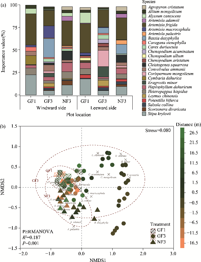
Fig. 3 Responses of species composition to different enclosure treatments (GF1, GF3, and NF3). (a), differences in the importance values of plant species on the windward and leeward sides of fences (the complete data are shown in Tables S1-3); (b), nonmetric multidimensional scaling (NMDS) of species composition, with dispersion ellipses at 95% confidence intervals added. PERMANOVA, permutational multivariate analysis of variance. Ellipse labels represent the 3 enclosure treatments, and the top 20 plant species points in terms of abundance are reflected in the figure. Distance indicates the distance from the sample plots to the fences.

3.2 Vegetation coverage, plant height, aboveground biomass, species richness, and plant density under different enclosure treatments

Vegetation coverage, aboveground biomass, species richness, and plant density were all significantly affected by the duration of GF (Table S4). Specifically, vegetation coverage, aboveground biomass, and species richness increased significantly in GF3 compared to GF1 by 8.15%, 109.238 g/m2, and 1.408 species/m2, respectively. Conversely, compared to NF3, these increases were 4.98%, 42.495 g/m2, and 1.015 species/m2, respectively, and were not statistically significant (Table S4).
The confirmed existence of the edge effects of fences, which caused heterogeneity in vegetation recovery, led us to undertake a quantitative analysis. Vegetation exhibited a nonlinear response to the distance from the fence, showing a consistent trend as it moved from the windward side to the leeward side, with most influencing initially increasing before gradually declining (Fig. 4). The fitted coefficient of distance in GF3 showed the greatest magnitude, indicating the most profound edge effects, with a significant increase stopping at 6.5 m (plant height), 11.5 m (vegetation coverage and aboveground biomass), and 26.5 m (species richness) on the leeward side. Vegetation coverage and aboveground biomass in GF1 gradually declined from the edge of the leeward side, with no significant difference observed at 16.5 and 11.5 m, respectively. However, no significant differences were observed among vegetation parameters at various distances in NF3 (Fig. 4).
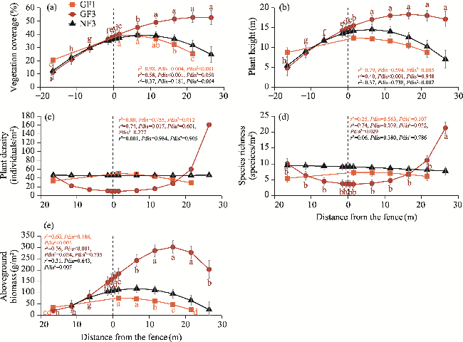
Fig. 4 Comparison of vegetation coverage (a), plant height (b), plant density (c), species richness (d), and aboveground biomass (e) at the interface between the windward and leeward sides of different enclosure treatments. Different lowercase letters indicate significant differences in means (P>0.05). Bars mean standard errors. Positive distances indicate sample plots within the enclosure area on the leeward side of the fences, and negative distances indicate sample plots within the grazing area on the windward side of the fences. Marginal r² refers to the fixed effects only. 'Pdis', 'Pdis2', and 'Ppdis3' represent significance tests for the distance, squared distance, and cubic distance from the fences, respectively. The abbreviations are the same in the following figures.

3.3 Soil physical and chemical properties under different enclosure treatments

The duration of GF and the presence of hanging grasses significantly influenced all the investigated soil physical and chemical properties, except SOC and SWC (Table S4). Along the transects, soil texture exhibited distinct patterns in response to the presence of hanging grasses, particularly evident in the region ranging from -1.5 to 6.5 m (Fig. 5). Here, sand content had positive edge effects when grasses hanging on the fences and negative edge effects when no grasses hanging on the fences. Far away from the fences, no significant differences were observed between the windward side interior (-16.5 m) and the leeward side interior (26.5 m). SOC and AP contents showed substantial distance impacts in GF3, with greater effects on the leeward side interior than on the windward side interior. However, SOC declined in the fence edge area. Meanwhile, AP content was significantly enriched. Furthermore, significant edge effects were observed for soil pH and AK content in NF3.
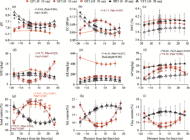
Fig. 5 Comparison of soil physical and chemical properties at the interface between the windward and leeward sides of fences under different enclosure treatments. (a), pH; (b), electrical conductivity (EC); (c), soil water content (SWC); (d), soil organic carbon (SOC) content; (e), available potassium (AK) content; (f), available phosphorus (AP) content; (g), sand content; (h), silt content; (i), clay content. Positive distances indicate sample plots within the enclosure area on the leeward side of the fence, and negative distances indicate sample plots within the grazing area on the windward side of the fence. Different lowercase letters indicate significant differences in means (P>0.05). Bars mean standard errors. Only model r2 values with P<0.05 are labeled in the figure; full model results are provided in Table S4. 'Psoil depth' indicates the significance of soil depth on soil physical and chemical properties. The abbreviations are the same in the following figures.

3.4 Relationship between environmental factors and vvegetation ccharacteristics under different enclosure treatments

The CCA results showed that the combined constrained variables explained 37.66% of the total variation in species composition, with the first two axes explaining 32.55% and 17.52%, respectively (Fig. 6a). The relationship between species composition and environmental factors had a strong correlation (adjusted R2=0.27), but to varying degrees among the different enclosure treatments. Species composition in GF1, NF3, and areas distant from GF3 exhibited a positive correlation with SOC and AP contents. However, in GF3 closer to the fence (-6.5 to 11.5 m), where surface sand had higher accumulation, there was a stronger correlation of species composition with EC, pH, and sand content. The variation partitioning results highlighted that plot factors, including the distance from the fence, the duration of GF, and the presence of hanging grasses, affected species composition (15.04%) and statistically outweighed the soil physical and chemical properties (3.22% and 1.65%, respectively) (Fig. 6b).
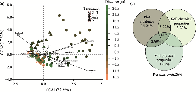
Fig. 6 Impacts of different environmental factors on species composition. (a), canonical correspondence analysis (CCA) of species composition at varying distances from the fence under different enclosure treatments; (b), contributions of different groups of environmental factors to species composition calculated by variation partitioning. Arrows represent the nine significant environmental factors selected for forward selection. "Treatment" represents the three different enclosure treatments: GF1, GF3, and NF3. "Thickness" denotes sand accumulation thickness. "Distance-Thickness" represents the interaction between distance from the fence and sand accumulation thickness. Note that factors with contributions to the total variance less than 0.0 are not shown.
SEM analysis was used to investigate the direct and indirect effects of enclosure measures and soil physical and chemical properties on vegetation coverage and plant density (Fig. 7a and b, respectively). The distance from the fence, sand accumulation thickness, and soil physical and chemical properties directly affected vegetation coverage, exhibiting a significant positive correlation. Different enclosure treatments did not directly affect vegetation coverage but exerted an indirect influence by altering soil physical and chemical properties (Fig. 7a). The only factor that was significantly negatively correlated with plant density was sand accumulation thickness. Soil physical and chemical properties did not considerably affect plant density, although sand accumulation thickness and enclosure treatments had a significant influence on this vegetation parameter (Fig. 7b).
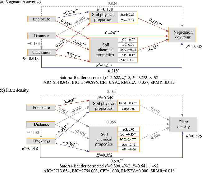
Fig. 7 Impacts of different environmental factors on vegetation coverage (a) and plant density (b) based on structural equation modelling (SEM). Boxes represent the environmental factors included in the model. Arrows indicate the paths, with the numbers on the paths representing standardized regression weights (the thicker the lines, the greater the weights). Solid arrows represent significant paths, with red solid arrows indicating positive effects, blue solid arrows indicating negative effects, and grey dashed arrows indicating non-significant paths. The significances along the paths at P<0.05, P<0.01, and P<0.001 levels are indicated by *, **, and ***, respectively. The standardized estimates and significance are displayed within each soil physical and chemical property box. The total explained variance of the environmental factors (R²) is marked near the box. χ2, chi-square; df, degree of freedom; n, sample size; AIC, Akaike information criterion; BIC, Bayesian information criterion; CFI, comparative fit index; RMSEA, root mean square error of approximation; SRMR, standardized root mean square residual.

4 Discussion

4.1 Vegetation changes in response to hanging grass fence enclosure

Fencing facilities such as edges for grassland enclosures lead to changes in richness, distribution, and growth rates of plant species (Wang et al., 2021). Tumbleweed accumulation and suspension on the fences would significantly intensify the biological differences between the grassland's interior and edge areas. This is because of the exclusion of grazing disturbances and the edge effects created by linear barriers. Taxa that are reduced or degraded during grassland degradation, such as Chenopodium album and Artemisia scoparia, can regenerate once harmful factors, such as grazing and animal trampling are removed (McDonald et al., 2019). Perennial palatable grasses such as Leymus chinensis had increased dominance within the enclosed area. Conversely, prostrate plants, such as Haplophyllum dahuricum and Heteropappus hispidus, had increased dominance outside the fences. This is consistent with the findings of Díaz et al. (2007) on the adaptive responses of low-growing plants to grazing. The higher vegetation coverage within the fence enclosure may enhance seed deposition, primarily facilitated by wind dispersal (Soons et al., 2004; Rotundo et al., 2015). This can benefit light and winged seeds such as Salsola collina, Corispermum mongolicum, and Eragrostis minor, which are more prevalent in the edge areas adjacent to the fences because the hanging grasses on the fences reduce wind speed on the leeward side. Nonetheless, following three years of hanging grass fence enclosure, the edge areas underwent a sharp decrease in species richness as a result of frequent disruptions caused by the entangled grasses on the fences and wind-blowing sand movement, with pioneer species such as Bassia dasyphylla dominating these areas. Sizer et al. (2000) also noted that the primary source of edge-recolonising species is the pioneer species within the seed bank established before edge formation.
Short-term enclosures with various fencing treatments have positively impacted parameters reflecting vegetation growth, such as vegetation coverage and aboveground biomass, a typical response to excluding grazing (Zhang et al., 2019; Liu et al., 2023). However, most vegetation features in the edge areas of fences have shown more significant responses to the presence of hanging grass fences and the duration of the enclosure than to the internal environment on both sides of fences. The edge effects of artificially constructed linear barriers, such as shelterbelts and hedgerows, have been documented in some ecosystems (Sitzia et al., 2013; Schopke et al., 2023). However, quantifying the edge effects of hanging grass fences is still rare (Wang et al., 2021). The changes in vegetation may be due to substantial structural modifications in the original fences caused by hanging grasses, which reduce the fences' porosity. This alteration could create gradient changes along the distance from the fence for microclimatic factors such as wind and light, potentially leading to differences in vegetation recovery at smaller scales (Pohlman et al., 2009; Wilkerson, 2014). Increased light on the leeward side creates favourable conditions for vegetation growth (Wang et al., 2021). Lower wind speeds establish a relatively stable microclimate around the vegetation, maintaining suitable temperature and humidity levels that support the growth and development of plants (Hamm and Drossel, 2017). Conversely, high wind speeds can disrupt these microclimates, leading to unstable environmental conditions.

4.2 Soil physical and chemical properties in response to hanging grass fence enclosure

Enclosure measures show considerable potential for rehabilitating degraded grasslands, particularly in environments susceptible to soil erosion, such as sandy grasslands (Matthews et al., 2017; Zhang et al., 2019). Inter-annual changes in wind speed can profoundly affect the occurrence and intensity of wind erosion and dust emissions (Shinoda et al., 2011). With increased wind speed, the likelihood of more frequent windblown sand activity increases, driven by the heightened sensitivity of temperate grasslands to climate variations. Conducted in moderately to severely degraded desert steppe in Central Mongolia (Meng et al., 2021), our study has shown changes in soil texture during the early stages of GF. We observed a significant increase in sand content within a 6.5 m range on the leeward side. This result contradicts the conclusions of Wang et al. (2021), who found no substantial impact of wind erosion or dust storms on the spatial distribution of soil texture components around fencing facilities, potentially because of the less prominent effect of fencing facilities. This also highlights how the structural changes in hanging grass fences from the original fencing structure resemble a sand barrier with a finer density in the lower part and a coarser density in the upper part. This potentially influences nearby soil physical and chemical properties by decelerating wind speed and trapping windblown sand and tumbleweeds. Significant variations in SOC, EC, and AP were observed at different distances from the fence. During the initial enclosure, the hanging grass fences contributed to a slight accumulation of SOC in the desert steppe (Wang et al., 2021). This is potentially due to the increased litter and nutrient release from vegetation restoration (Zhang et al., 2018; Wang et al., 2023) and tumbleweed remnants on the fences. However, sand accumulation may affect the transformation of plant debris into organic carbon within the soil (Pulido et al., 2018). The reduced wind speed on the leeward side of hanging grass fences may have diminished soil moisture evaporation (Teng et al., 2014) and enhanced soil water retention (Liang et al., 2021). However, this process is complex and warrants further investigation.

4.3 Key environmental factors affecting vegetation parameters

Non-biological edge effects, such as microclimate and soil physical and chemical properties, play a significant role in causing heterogeneity in vegetation recovery (Matlack, 1993; Yates et al., 2000). However, the primary environmental factors with the strongest influence in this scenario remain unclear. In this study, the influence of hanging grass fences on the topsoil led to changes in soil texture, nutrients, and organic matter content, thereby affecting the quantity and distribution of vegetation. The microclimate generated by linear barriers might be an underlying factor driving vegetation changes (Cleugh and Hughes, 2002), potentially enhancing vegetation habitats near fences owing to temperature and humidity alterations (Gasperini et al., 2021). Microclimate measurements were not directly obtained in this study, while indirect evidence was derived from the profound modification of the microtopography on both sides of the fences that resulted from the substantial shift in windblown sand retention caused by hanging grass fences. Environmental factors such as sand content, EC, and sand accumulation thickness are pivotal determinants of changes in species composition and plant density. The leeward side of sand barriers often exhibits significant sand accumulation, which can reduce wind erosion on the ground surfaces (Zhang et al., 2016; Xi et al., 2023). Similar to the movement observed in gas-solid two-phase flow, hanging grass fences trap sand grains but may also cause wind-dispersed seeds commonly found in grasslands to settle on the wind shadow area of the leeward side owing to its wind attenuation effect, potentially increasing the local soil seed bank (Luo et al., 2019). A relevant study confirmed a significant positive correlation between the richness of wind-dispersed plant species and vegetation hedges composed of grass matrices (Wilkerson, 2014).

4.4 Implication from potential restorative effects of hanging grass fences

Considering the extensive environment of Mongolian grasslands, hanging grass fences have a relatively limited range of effects. The observed ecological effects appear to be short term and are primarily influenced by wind-blown sand deposition. Long-term ecological implications require further observations and assessment. However, the immediate and significant effects of hanging grass fences on local ecological restoration and soil conservation should not be overlooked. Due to the constraints placed on pastoralists' efforts and the organization and administration of ecological restoration projects due to the tragedy of the commons, special consideration is required in Mongolia's community-based institutions for rangeland management (Bruegger et al., 2014). Emphasis should be placed on severely degraded areas, such as settlement peripheries, roadside areas, and water sources, which are commonly frequented by grazing activities and are often subjected to trampling by cattle and sheep (Fernandez-Gimenez, 2000). Adjusting the fence direction and grid density to suit the prevailing wind patterns and creating hanging grass fences is recommended in these areas. This approach supports wind erosion mitigation, ecological restoration, and economic savings. During severe weather that causes extensive livestock losses, hanging grass fences may be essential sites for grazing, providing shelter from wind and snow and offering some fodder once vegetation recovers.

5 Conclusions

Hanging grass fences and the non-negligible presence of grassland enclosures with tumbleweed dispersal have considerable importance in vegetation recovery and soil physical and chemical properties in degraded grasslands. Their influence extends beyond the exclusion of grazing disturbances and encompasses the edge effects produced by linear barriers. Our study has provided critical insights into hanging grass fences in degraded desert steppe in Central Mongolia. As common barriers in vast grasslands, fences introduce an uneven vegetation distribution and soil physical and chemical properties after grasses hanging on the fences. The vegetation parameters and soil physical and chemical properties responded nonlinearly to fence proximities. Uneven spatial vegetation recovery may be attributed to the accumulation of soil nutrients, sand content, seed banks near the fences, and microclimate change. Without microtopographic change, nutrient accumulation, such as SOC and AK, drives differentiation in species composition and vegetation coverage. As the enclosure duration increased, distinct accumulations of sand dunes near hanging grass fences affected factors such as sand content, EC, and sand accumulation thickness, which are crucial for determining changes in species composition and plant density. These findings can provide key insights into the restoration and management of grassland ecosystems. And they may offer new directions for practical exploration and ecological conservation such as protective measures in areas prone to sand damage, serving as barriers for livestock during disasters and providing forage after vegetation regreening. Further studies on the role of linear barriers in grassland restoration are required to better leverage their edge effects, which play a substantial role in the recovery of grassland ecosystems on the Mongolian Plateau and beyond temperate grasslands.

Conflict of interest

The authors declare that they have no known competing financial interests or personal relationships that could have appeared to influence the work reported in this paper.

Acknowledgements

This study was supported by the Third Xinjiang Scientific Expedition and Research Program (2021xjkk0305), the Strategic Priority Research Program of the Chinese Academy of Sciences (XDA2003020201), and the Key Intergovernmental Projects for International Scientific and Technological Innovation Cooperation of the National Key Research and Development Program of China (2017YFE0109200). We appreciate the valuable support provided by the assessment and mapping desertification research team of the Institute of Geography and GeoEcology, Mongolian Academy of Sciences, Mongolia, during our field sampling work.

Author contributions

Conceptualisation: LI Shengyu, XU Xinwen; Methodology: MIAO Jiamin, LIU Guojun; Investigation: LIU Guojun, WANG Haifeng, FAN Jinglong, Khaulanbek AKHMADI, MIAO Jiamin; Formal analysis: MIAO Jiamin, WANG Haifeng, FAN Jinglong; Writing - original draft preparation: MIAO Jiamin; Writing - review and editing: LI Shengyu, MIAO Jiamin; Funding acquisition: LI Shengyu; Supervision: LI Shengyu, XU Xinwen. All authors approved the manuscript.

Appendix

Table S1 Relative importance values of species at different distances from fences in the first year of enclosure with hanging grass fences (GF1)
Species Relative importance value (%)
-16.5 m 1.5 m 6.5 m 11.5 m 16.5 m 21.5 m
Bassia dasyphylla 0.00 0.00 0.00 0.74 0.00 0.00
Eragrostis minor 0.90 3.48 0.00 0.00 0.00 0.00
Chenopodium acuminatum 0.00 0.00 0.00 0.00 0.00 0.00
Salsola collina 0.00 3.14 1.13 0.00 0.00 0.00
Corispermum mongolicum 0.00 1.43 0.97 0.00 0.00 0.00
Artemisia frigida 34.47 29.70 25.27 34.94 38.19 32.57
Convolvulus ammanii 5.00 0.78 0.00 0.00 1.69 0.00
Carex duriuscula 0.00 0.00 0.00 0.00 0.00 1.27
Chenopodium aristatum 0.00 0.00 0.00 0.00 0.00 0.00
Allium mongolicum 3.76 0.00 3.71 3.75 0.00 5.70
Haplophyllum dahuricum 2.95 7.86 6.57 4.05 7.87 7.10
Setaria viridis 0.00 0.00 0.00 0.00 0.00 0.00
Astragalus sp. 0.00 0.00 0.00 0.00 0.00 0.00
Chenopodium album 0.00 2.61 8.06 3.96 0.00 0.00
Stipa krylovii 22.32 19.99 14.85 14.79 19.10 19.74
Alyssum canescens 5.94 15.62 4.49 13.50 13.16 11.33
Cleistogenes squarrosa 0.00 0.00 0.00 0.00 0.00 0.00
Leymus chinensis 0.00 1.86 0.00 0.00 0.00 0.00
Sibbaldianthe adpressa 0.00 0.00 0.00 0.00 0.00 0.00
Tribulus terrestris 0.00 0.00 0.00 0.00 0.00 0.00
Caragana stenophylla 4.55 2.11 0.00 3.39 0.00 2.80
Allium polyrhizum 1.63 0.00 0.00 0.00 0.00 0.00
Artemisia scoparia 0.00 0.00 2.36 0.00 5.70 0.00
Heteropappus hispidus 7.62 2.97 6.72 7.86 8.63 5.69
Caragana microphylla 0.00 0.00 0.00 0.00 0.00 0.00
Asparagus dahurica 0.00 2.00 3.21 0.00 0.00 0.00
Artemisia macrocephala 2.30 0.00 9.81 3.51 0.00 3.15
Oxytropis sp. 0.00 0.00 0.00 0.00 0.00 0.00
Cymbaria dahurica 9.75 0.00 0.00 0.00 0.00 3.50
Potentilla bifurca 0.00 0.00 2.41 7.00 2.72 7.14
Agropyron cristatum 0.00 7.58 7.35 0.00 0.00 0.00
Scorzonera sp. 0.00 0.00 0.00 0.00 0.00 0.00
Carex sp. 0.00 0.00 0.00 0.00 0.00 0.00
Artemisia palustris 0.00 0.00 1.60 0.00 0.00 0.00
Artemisia adamsii 0.00 0.00 1.49 2.51 0.00 0.00

Note: Positive distances indicate sample plots within the enclosure area on the leeward side of the fences, and negative distances indicate sample plots within the grazing area on the windward side of the fences.

Table S2 Relative importance values of species at different distances from fences in the third year of enclosure with hanging grass fences (GF3)
Species Relative importance value (%)
-16.5 m -11.5 m -6.5 m -1.5 m -0.5 m 0.5 m 1.5 m 6.5 m 11.5 m 16.5 m 21.5 m 26.5 m
Bassia dasyphylla 57.22 47.38 0.00 0.61 0.00 12.87 13.30 0.00 3.95 5.21 3.97 5.78
Eragrostis minor 10.30 8.87 0.36 0.00 0.00 42.85 15.23 10.71 6.93 5.97 0.00 0.00
Chenopodium acuminatum 0.00 0.00 3.80 2.48 0.00 7.33 5.91 1.88 4.45 4.99 1.94 3.56
Salsola collina 0.00 6.75 2.27 0.00 1.77 6.81 5.01 0.00 2.51 2.08 2.90 1.55
Corispermum mongolicum 4.75 6.90 0.00 0.00 0.00 24.81 47.39 11.56 21.05 18.70 1.52 2.39
Artemisia frigida 1.15 0.00 29.14 31.28 25.59 0.00 0.00 19.44 21.60 26.51 31.80 36.13
Convolvulus ammanii 0.00 0.00 5.81 9.78 18.16 0.00 0.00 4.17 3.48 4.85 7.87 5.00
Carex duriuscula 0.00 0.00 7.41 6.51 2.78 0.00 0.00 5.47 3.44 4.60 11.30 8.85
Chenopodium aristatum 0.00 0.00 0.00 0.00 0.00 7.74 7.11 2.42 4.83 0.59 1.58 0.00
Allium mongolicum 0.00 0.00 7.72 4.01 1.49 0.00 0.00 2.17 1.35 1.02 2.40 3.65
Haplophyllum dahuricum 0.00 0.00 6.81 4.16 10.12 0.00 0.00 4.60 2.13 3.69 0.83 0.00
Setaria viridis 0.00 0.00 0.00 0.00 0.00 0.00 2.41 0.00 0.00 3.73 0.00 0.00
Astragalus sp. 0.00 0.00 0.00 3.19 4.83 0.00 0.00 0.77 0.00 0.00 0.00 3.38
Chenopodium album 0.00 0.00 0.00 0.00 0.00 0.00 0.00 0.00 1.69 0.87 0.00 0.00
Stipa krylovii 0.00 0.00 10.24 3.06 10.89 0.00 0.00 3.24 4.05 6.22 10.74 9.89
Alyssum canescens 0.00 0.00 0.69 2.47 0.00 0.00 0.00 1.17 1.01 0.00 1.66 0.00
Cleistogenes squarrosa 2.15 0.00 2.36 3.78 2.83 0.00 0.00 0.00 0.00 0.48 1.93 0.38
Leymus chinensis 0.00 0.00 3.40 9.43 7.18 0.00 0.00 13.07 15.18 2.74 6.53 8.58
Sibbaldianthe adpressa 0.00 0.00 0.00 0.00 0.00 0.00 0.00 0.00 0.00 0.54 1.39 2.23
Tribulus terrestris 0.00 6.26 0.00 0.00 0.00 1.47 3.64 0.62 0.89 0.00 0.00 0.74
Caragana stenophylla 0.00 0.00 2.10 1.69 2.97 0.00 0.00 1.82 0.00 7.55 0.00 2.02
Allium polyrhizum 0.00 0.00 0.00 0.00 0.00 0.00 0.00 0.00 0.00 1.44 0.99 1.55
Artemisia scoparia 0.00 0.00 0.00 0.00 0.00 0.00 0.00 0.00 0.00 0.00 0.81 0.00
Heteropappus hispidus 0.00 0.00 1.24 7.51 5.04 0.00 0.00 8.29 0.00 0.00 1.00 3.55
Caragana microphylla 0.00 0.00 0.00 0.00 0.00 0.00 0.00 0.00 0.00 0.00 0.70 0.00
Asparagus dahurica 0.00 0.00 1.46 0.00 0.00 0.00 0.00 0.00 0.00 1.46 0.00 1.39
Artemisia macrocephala 22.81 23.84 7.97 7.60 4.30 0.00 0.00 3.91 0.00 0.00 0.00 0.00
Oxytropis sp. 0.00 0.00 1.05 0.00 0.00 0.00 0.00 0.00 0.00 0.00 0.00 0.00
Cymbaria dahurica 0.00 0.00 1.29 0.00 0.00 0.00 0.00 0.00 0.00 0.00 0.00 0.00
Potentilla bifurca 0.00 0.00 5.77 1.41 0.00 0.00 0.00 2.94 2.30 1.03 4.15 0.75
Agropyron cristatum 0.00 0.00 0.00 0.00 1.34 0.00 0.00 0.00 0.00 0.00 4.70 0.00
Scorzonera sp. 0.00 0.00 2.06 1.02 0.00 0.00 0.00 0.89 0.00 0.00 0.00 0.92
Carex sp. 0.00 0.00 0.00 0.00 0.72 0.00 0.00 0.85 0.00 0.00 0.00 0.00
Artemisia palustris 0.00 0.00 3.17 0.00 0.00 0.00 0.00 0.00 0.00 0.00 0.00 0.00
Artemisia adamsii 1.62 0.00 0.00 0.00 0.00 0.00 0.00 0.00 0.00 0.00 0.00 0.00

Note: Positive distances indicate sample plots within the enclosure area on the leeward side of the fences, and negative distances indicate sample plots within the grazing area on the windward side of the fences.

Table S3 Relative importance values of species at different distances from fences in the third year of enclosure with non-hanging grass fences (NF3)
Species Relative importance value (%)
-16.5 m -11.5 m -6.5 m -1.5 m -0.5 m 0.5 m 1.5 m 6.5 m 11.5 m 16.5 m 21.5 m 26.5 m
Bassia dasyphylla 3.47 0.00 0.00 0.00 0.00 40.88 17.53 6.66 0.00 8.25 0.00 0.00
Eragrostis minor 0.00 0.00 0.00 0.00 0.00 0.00 0.00 0.00 0.00 0.00 0.00 0.00
Chenopodium acuminatum 2.76 0.00 0.00 0.00 0.00 0.00 1.96 0.00 0.00 2.21 0.00 0.00
Salsola collina 2.99 0.00 0.00 1.69 1.70 2.96 5.80 9.26 0.00 1.09 1.40 0.00
Corispermum mongolicum 2.02 0.00 0.00 0.00 0.00 10.97 3.99 0.00 0.00 0.00 0.00 0.00
Artemisia frigida 18.03 30.11 25.68 25.11 36.72 4.37 22.05 20.85 23.27 40.23 36.99 22.71
Convolvulus ammanii 0.00 0.00 7.63 5.24 0.00 0.00 0.00 0.00 0.00 0.00 10.79 14.09
Carex duriuscula 0.00 0.00 5.22 6.09 0.00 0.00 0.00 1.24 1.53 1.94 0.00 2.20
Chenopodium aristatum 0.00 0.00 0.00 0.00 0.00 0.00 0.00 0.00 0.00 0.00 0.00 0.00
Allium mongolicum 1.78 3.53 4.54 0.00 2.42 0.00 0.00 0.00 1.92 11.66 3.99 2.11
Haplophyllum dahuricum 9.69 6.98 11.60 13.18 7.53 10.46 10.01 1.73 10.28 3.18 0.00 9.49
Setaria viridis 0.00 0.00 0.00 0.00 0.00 1.74 0.00 0.00 0.00 0.00 0.00 0.00
Astragalus sp. 0.00 0.00 0.00 0.00 0.00 0.00 2.22 2.38 0.91 0.00 0.00 2.34
Chenopodium album 0.00 0.00 0.00 0.00 0.00 1.37 1.69 0.00 0.00 0.00 0.00 0.00
Stipa krylovii 7.40 19.59 12.17 6.26 9.81 7.10 8.96 12.42 11.10 2.01 12.75 11.69
Alyssum canescens 1.52 6.05 2.46 3.04 5.97 0.84 0.00 0.00 1.33 0.00 0.00 0.00
Cleistogenes squarrosa 7.07 8.21 16.19 11.00 5.68 0.00 0.00 9.10 16.70 4.02 8.61 15.09
Leymus chinensis 0.00 0.00 0.00 0.00 5.81 0.00 0.00 0.00 0.00 0.00 1.78 0.00
Sibbaldianthe adpressa 0.00 0.00 0.00 0.00 0.00 0.00 0.00 0.00 0.00 0.00 0.00 0.00
Tribulus terrestris 0.00 0.00 0.00 0.00 0.00 0.00 0.00 0.00 0.00 0.00 0.00 0.00
Caragana stenophylla 3.07 4.28 0.00 0.00 0.00 0.00 0.00 0.00 0.00 0.00 0.00 0.00
Allium polyrhizum 0.00 0.00 0.00 2.52 0.00 0.00 0.00 0.00 0.00 0.00 0.00 4.27
Artemisia scoparia 0.00 0.00 0.00 0.00 0.00 0.00 0.00 0.00 0.00 0.00 0.00 0.00
Heteropappus hispidus 7.06 4.55 3.75 11.05 11.66 2.14 3.69 0.00 9.65 8.89 5.51 7.39
Caragana microphylla 0.00 0.00 0.00 0.00 0.00 0.00 0.00 0.00 0.00 0.00 0.00 0.00
Asparagus dahurica 0.00 2.86 3.69 0.00 5.17 0.00 0.00 0.00 0.00 5.21 0.00 0.00
Artemisia macrocephala 2.92 0.00 0.00 0.00 0.00 2.38 0.00 0.00 0.00 0.00 0.00 0.00
Oxytropis sp. 0.00 0.00 0.00 0.00 0.00 0.00 0.00 0.00 0.00 0.00 0.00 0.00
Cymbaria dahurica 0.00 0.00 0.00 0.00 0.00 0.00 0.00 0.00 0.00 0.00 0.00 4.50
Potentilla bifurca 0.00 0.00 0.00 0.00 0.00 0.00 0.00 0.00 0.00 8.62 11.91 0.00
Agropyron cristatum 5.45 1.68 2.33 6.58 1.91 4.43 14.73 2.51 6.79 2.69 3.00 0.00
Scorzonera sp. 1.87 3.24 4.72 8.24 5.64 0.00 0.00 0.00 8.71 0.00 3.27 4.11
Carex sp. 0.00 0.00 0.00 0.00 0.00 0.00 0.00 0.00 0.00 0.00 0.00 0.00
Artemisia palustris 6.02 0.00 0.00 0.00 0.00 0.00 10.29 22.63 0.00 0.00 0.00 0.00
Artemisia adamsii 16.89 8.95 0.00 0.00 0.00 10.37 1.55 11.21 7.82 0.00 0.00 0.00

Note: Positive distances indicate sample plots within the enclosure area on the leeward side of the fences, and negative distances indicate sample plots within the grazing area on the windward side of the fences.

Table S4 Effects of the duration of enclosure with hanging grass fences (GF) and the presence of hanging grasses on vegetation parameters and soil physical and chemical properties based on the linear mixed model (LMM)
Variable Goodness-of-fit Intercept Distance from the fence (m) DiffGF1-GF3 SAT Distance-Year 2021 Soil depth
(0-10 cm)
Marginal r² Conditional r²
GF1 vs. GF3
Vegetation coverage 0.525 0.585 31.397*** (3.563) 0.241 (0.186) 8.150* (3.684) 0.096 (0.155) 0.798** (0.241) -
Plant height 0.460 0.546 10.867*** (1.342) 0.037 (0.007) 2.324 (1.322) 0.067 (0.056) 0.295** (0.086) -
Aboveground biomass 0.629 0.670 55.865* (23.022) -0.049 (1.248) 109.238*** (24.609) 2.075 (1.041) 6.862*** (1.615) -
Species richness 0.557 0.560 6.495*** (1.052) 1.004 (1.003) 1.408*** (1.007) 0.980*** (1.003) 0.996 (1.004) -
Plant density 0.904 0.904 46.390*** (1.058) 1.001 (1.006) 0.898 (1.094) 0.975*** (1.002) 0.999 (1.008) -
pH 0.414 0.586 6.617*** (0.126) -0.001 (0.005) 0.490*** (0.101) 0.007 (0.004) 0.011 (0.007) -
SOC 0.256 0.320 10.220*** (0.580) 0.007 (0.030) -0.413 (0.650) -0.048 (0.030) -0.101* (0.043) -
EC 0.459 0.529 0.038** (0.008) 0.000 (0.000) 0.021* (0.009) 0.002*** (0.000) 0.001 (0.001) -
AP 0.656 0.913 32.226*** (2.647) -0.054 (0.166) -13.076*** (2.482) 0.178** (0.060) 0.421 (0.216) -
AK 0.955 0.972 434.036*** (17.475) -3.688* (1.613) -295.078*** (23.429) 0.583 (0.576) 3.920 (2.101) -
Sand content 0.344 0.356 77.912*** (1.492) 0.032 (0.099) -4.051* (1.904) 0.363*** (0.082) 0.163 (0.128) -
Silt content 0.336 0.350 11.714*** (1.234) -0.042 (0.081) 3.581* (1.568) -0.290*** (0.068) -0.114 (0.105) -
Clay content 0.363 0.669 10.096*** (0.588) 0.012 (0.050) -0.252 (0.737) -0.052** (0.018) -0.053 (0.066) -
Vegetation coverage 0.369 0.389 32.035*** (3.293) 0.247 (0.220) 4.982 (3.968) -0.125 (0.093) 0.654* (0.271) -
Plant height 0.315 0.325 11.714*** (1.171) 0.023 (0.083) 0.133 (1.472) 0.093* (0.035) 0.285** (0.103) -
Aboveground biomass 0.383 0.471 102.824** (26.800) 0.472 (1.377) 42.495 (26.267) 0.411 (0.587) 5.777** (1.698) -
Species richness 0.638 0.672 8.933*** (1.081) 0.995 (1.004) 1.015 (1.086) 0.980*** (1.002) 1.006 (1.005) -
Plant density 0.666 0.674 46.109*** (1.100) 1.000 (1.007) 0.905 (1.124) 0.971*** (1.003) 1.002 (1.008) -
pH 0.114 0.288 7.386*** (0.127) -0.015** (0.005) -0.211* (0.091) 0.003 (0.002) 0.022*** (0.006) -0.148* (0.067)
SOC 0.215 0.219 10.038*** (0.492) -0.028 (0.032) 0.636 (0.557) -0.080*** (0.013) 0.033 (0.039) -0.408 (0.457)
EC 0.259 0.299 0.078*** (0.012) -0.002** (0.001) -0.025* (0.012) 0.002*** (0.000) 0.002* (0.009) 0.006 (0.001)
AP 0.308 0.512 16.987*** (3.454) 0.166 (0.370) -2.288 (3.931) 0.273*** (0.065) 0.276 (0.454) 4.070* (1.909)
AK 0.366 0.382 69.350*** (9.090) 0.573 (0.521) 44.403*** (9.564) 0.903*** (0.221) 0.232 (0.643) 26.387*** (7.516)
Sand content 0.489 0.493 73.785*** (1.238) -0.179 (0.232) 5.364** (2.002) 0.145*** (0.037) 0.260 (0.361) -2.150 (1.195)
Silt content 0.425 0.435 13.740*** (0.990) 0.164 (0.180) -3.015 (1.587) -0.105*** (0.029) −0.208 (0.221) 1.741 (0.927)
Clay content 0.486 0.486 12.520*** (0.408) 0.015 (0.079) -2.444*** (0.664) -0.039** (0.012) -0.052 (0.097) 0.409 (0.407)
SWC 0.004 0.059 4.007 (0.125) 0.002 (0.006) 0.039 (0.121) 0.001 (0.003) -0.001 (0.008) 0.002 (0.093)

Note: The goodness of fit, intercept, coefficient, and standard error (value in the parenthese) of LMM are presented. DiffGF1-GF3, the difference between GF3 and GF1; DiffGF1-NF3, the difference between GF3 and NF3; SAT, sand accumulation thickness; Distance-Year 2021, interaction effects with fence distance and year. EC, electrical conductivity; SWC, soil water content; SOC, soil organic carbon; AK, available potassium; AP, available phosphorus. "-" indicates that the variable is not included in the model calculation. *, **, and *** mean coefficients outside the 95.0%, 99.0% and 99.9% confidence intervals, respectively.

[1]
Allan E, Manning P, Alt F, et al. 2015. Land use intensification alters ecosystem multifunctionality via loss of biodiversity and changes to functional composition. Ecology Letters, 18(8): 834-843.

[2]
Bai Y F, Cotrufo M F. 2022. Grassland soil carbon sequestration: Current understanding, challenges, and solutions. Science, 377(6606): 603-608.

[3]
Baker D V, Beck K G. 2008. The weed tunnel: Building an experimental wind tunnel. Weed Technology, 22(3): 549-552.

[4]
Bao S. 2000. Soil and Agricultural Chemistry Analysis. Beijing: China Agriculture Press, 14-209. (in Chinese)

[5]
Bates D, Mächler M, Bolker B, et al. 2015. Fitting linear mixed-effects models using lme4. Journal of Statistical Software, 67(1): 1-48.

[6]
Becker D A. 1978. Stem abscission in tumbleweeds of the Chenopodiaceae: Kochia. American Journal of Botany, 65(4): 375-383.

[7]
Bell L W, Kirkegaard J A, Swan A, et al. 2011. Impacts of soil damage by grazing livestock on crop productivity. Soil & Tillage Research, 113(1): 19-29.

[8]
Boutin C, Baril A, Martin P A. 2008. Plant diversity in crop fields and woody hedgerows of organic and conventional farms in contrasting landscapes. Agriculture, Ecosystems & Environment, 123(1-3): 185-193.

[9]
Bruegger R A, Jigjsuren O, Fernández-Giménez M E. 2014. Herder observations of rangeland change in Mongolia: indicators, causes, and application to community-based management. Rangeland Ecology & Management, 67(2): 119-131.

[10]
Burst M, Chauchard S, Dambrine E, et al. 2020. Distribution of soil properties along forest-grassland interfaces: Influence of permanent environmental factors or land-use after-effects? Agriculture, Ecosystems & Environment, 289: 106739, doi: 10.1016/j.agee.2019.106739.

[11]
Cardelús C L, Mekonnen A B, Jensen K H, et al. 2020. Edge effects and human disturbance influence soil physical and chemical properties in Sacred Church Forests in Ethiopia. Plant and Soil, 453: 329-342.

[12]
Cleugh H A, Hughes D E. 2002. Impact of shelter on crop microclimates: A synthesis of results from wind tunnel and field experiments. Australian Journal of Experimental Agriculture, 42(6): 679-701.

[13]
Díaz S, Lavorel S, McIntyre S, et al. 2007. Plant trait responses to grazing-a global synthesis. Global Change Biology, 13(2): 313-341.

[14]
Du C J, Jing J, Shen Y, et al. 2020. Short-term grazing exclusion improved topsoil conditions and plant characteristics in degraded alpine grasslands. Ecological Indicators, 108: 105680, doi: 10.1016/j.ecolind.2019.105680.

[15]
Eldridge D J, Delgado-Baquerizo M. 2017. Continental-scale impacts of livestock grazing on ecosystem supporting and regulating services. Land Degradation & Development, 28(4): 1473-1481.

[16]
Ewers R M, Didham R K. 2006. Continuous response functions for quantifying the strength of edge effects. Journal of Applied Ecology, 43(3): 527-536.

[17]
Fernandez-Gimenez M E. 2000. The role of Mongolian nomadic pastoralists' ecological knowledge in rangeland management. Ecological Applications, 10(5): 1318-1326.

[18]
Feyisa K, Beyene S, Angassa A, et al. 2017. Effects of enclosure management on carbon sequestration, soil properties and vegetation attributes in East African rangelands. Catena, 159: 9-19.

[19]
Fox J, Weisberg S. 2019. An R Companion to Applied Regression (3rd ed.). Thousand Oaks, CA: Sage. [2024-01-03]. https://socialsciences.mcmaster.ca/jfox/Books/Companion/.

[20]
Gasperini C, Carrari E, Govaert S, et al. 2021. Edge effects on the realised soil seed bank along microclimatic gradients in temperate European forests. Science of the Total Environment, 798: 149373, doi: 10.1016/j.scitotenv.2021.149373.

[21]
Haddaway N R, Brown C, Eales J, et al. 2018. The multifunctional roles of vegetated strips around and within agricultural fields. Environmental Evidence, 7: 14, doi: 10.1186/s13750-018-0126-2.

[22]
Hamm M, Drossel B. 2017. Habitat heterogeneity hypothesis and edge effects in model metacommunities. Journal of Theoretical Biology, 426: 40-48

[23]
Hao G, Dong K, Yang N, et al. 2021. Both fencing duration and shrub cover facilitate the restoration of shrub-encroached grasslands. Catena, 207: 105578, doi: 10.1016/j.catena.2021.105587.

[24]
Hu Z Y, Ma Y Y, Jin Q J, et al. 2023. Attribution of the March 2021 exceptional dust storm in North China. Bulletin of the American Meteorological Society, 104(4): E749-E755.

[25]
Ju W L, Fang L C, Shen G T, et al. 2023. New perspectives on microbiome and nutrient sequestration in soil aggregates during long-term grazing exclusion. Global Change Biology, 30(1): e17027, doi: 10.1111/gcb.17027.

[26]
Khaulanbek A, Tsogtbaatar J, Khudulmur S. 2013. National Atlas on Desertification. Ulaanbaatar: Bembi-San, 2-5.

[27]
Kinar N J. 2017. Modeling blowing snow accumulation downwind of an obstruction: The Ohara Eulerian particle distribution equation. Water Resources Research, 53(5): 3557-3564.

[28]
Lenth R V. 2016. Least-squares means: The R package lsmeans. Journal of Statistical Software, 69(1): 1-33.

[29]
Li G, Qin J M, Yu H X, et al. 2022. Wind-tunnel experimental studies of the spatial snow distribution over grass and bush surfaces. Journal of Hydrodynamics, 34: 85-93.

[30]
Li S G, Tsujimura M, Sugimoto A, et al. 2006. Natural recovery of steppe vegetation on vehicle tracks in Central Mongolia. Journal of Biosciences, 31: 85-93.

[31]
Liang Y M, Gao Y, Wang R D, et al. 2021. Fungal community characteristics and driving factors during the decaying process of Salix psammophila sand barriers in the desert. PLoS ONE, 16(10): e0258159, doi: 10.1371/journal.pone.0258159

[32]
Liira J, Paal T. 2013. Do forest-dwelling plant species disperse along landscape corridors? Plant Ecology, 214: 455-470.

[33]
Liu C, Li H, Liu K S, et al. 2023. Vegetation characteristics of the main grassland types in China respond differently to the duration of enclosure: a meta-analysis. Agronomy-Basel, 13(3): 854, doi: 10.3390/agronomy13030854.

[34]
Luo J F, Deng D Z, Zhang L, et al. 2019. Soil and vegetation conditions changes following the different sand dune restoration measures on the Zoige Plateau. PLoS ONE, 14(9): e0216975, doi: 10.1371/journal.pone.0216975.

[35]
Ma W Y, Luo Y, Li F Q, et al. 2022. The influence of wind deflectors on the snow distribution in road cuttings during snowdrift. Cold Regions Science and Technology, 196: 103505, doi: 10.1016/j.coldregions.2022.103505.

[36]
Matlack G R. 1993. Microenvironment variation within and among forest edge sites in the Eastern United States. Biological Conservation, 66(3): 185-194.

[37]
Matthews J W, Molano-Flores B, Ellis J, et al. 2017. Impacts of management and antecedent site condition on restoration outcomes in a sand prairie. Restoration Ecology, 25(6): 972-981.

[38]
McDonald S E, Lawrence R, Kendal L, et al. 2019. Ecological, biophysical and production effects of incorporating rest into grazing regimes: A global meta-analysis. Journal of Applied Ecology, 56(12): 2723-2731.

[39]
Meng X Y, Gao X, Li S Y, et al. 2020. Spatial and temporal characteristics of vegetation NDVI changes and the driving forces in Mongolia during 1982-2015. Remote Sensing, 12(4): 603, doi: 10.3390/rs12040603.

[40]
Meng X Y, Gao X, Li S, et al. 2021. Monitoring desertification in Mongolia based on Landsat images and Google Earth Engine from 1990 to 2020. Ecological Indicators, 129: 107908, doi: 10.1016/j.ecolind.2021.107908.

[41]
Michels K K, Hotchkiss S C, Jonaitis E, et al. 2017. A new application of change point analysis reveals extensive edge effects on a temperate mixed forest. Applied Vegetation Science, 20(4): 651-661.

[42]
Munoz-Cerro E, Garcia-Duro J, Matinez-Ruiz C, et al. 2023. Soil amelioration induced by nurse shrubs in coal mines reclaimed to pastures and their synergistic effects with grazing. Agriculture, Ecosystems & Environment, 350: 108483, doi: 10.1016/j.agee.2023.108483.

[43]
Novaes L R, Calixto E S, Alves-de-Lima L, et al. 2022. Testing direct and indirect road edge effects on reproductive components of anemochoric plants. Landscape and Urban Planning, 218: 104291, doi: 10.1016/j.landurbplan.2021.104291.

[44]
Oksanen J, Blanchet F G, Friendly M, et al. 2020. Vegan: Community Ecology Package. R package version 2.5-7. [2023-09-01]. https://CRAN.R-project.org/package=vegan.

[45]
Pohlman C L, Turton S M, Goosem M. 2009. Temporal variation in microclimatic edge effects near powerlines, highways and streams in Australian tropical rainforest. Agricultural and Forest Meteorology, 149(4): 84-95.

[46]
Porensky L M. 2011. When edges meet: interacting edge effects in an African savanna. Journal of Ecology, 99(4): 923-934.

[47]
Pulido M, Schnabel S, Contador J F L, et al. 2018. The impact of heavy grazing on soil quality and pasture production in rangelands of SW Spain. Land Degradation & Development, 29(2): 219-230.

[48]
Ries L, Sisk T D. 2004. A predictive model of edge effects. Ecology, 85(11): 2917-2926.

[49]
Rosseel Y. 2012. Lavaan: An R package for structural equation modeling. Journal of Statistical Software, 48(2): 1-36.

[50]
Rotundo J L, Aguiar M R, Benech-Arnold R. 2015. Understanding erratic seedling emergence in perennial grasses using physiological models and field experimentation. Plant Ecology, 216: 143-156.

[51]
Sainnemekh S, Barrio I C, Densambuu B, et al. 2022. Rangeland degradation in Mongolia: A systematic review of the evidence. Journal of Arid Environments, 196: 104654, doi: 10.1016/j.jaridenv.2021.104654.

[52]
Sanaei A, Li M S, Ali A. 2019. Topography, grazing, and soil textures control over rangelands' vegetation quantity and quality. Science of the Total Environment, 697: 134153, doi: 10.1016/j.scitotenv.2019.134153.

[53]
Schopke B, Wesche K, Wulf M. 2023. Dry grasslands adjacent to organic fields have higher plant diversity-Even far into their interior. Agriculture, Ecosystems & Environment, 357: 108672, doi: 10.1016/j.agee.2023.108672.

[54]
Seddon A W R, Macias-Fauria M, Long P R, et al. 2016. Sensitivity of global terrestrial ecosystems to climate variability. Nature, 531: 229-232.

[55]
Shinoda M, Gillies J A, Mikami M, et al. 2011. Temperate grasslands as a dust source: Knowledge, uncertainties, and challenges. Aeolian Research, 3(3): 271-293.

[56]
Sitzia T, Trentanovi G, Marini L, et al. 2013. Assessment of hedge stand types as determinants of woody species richness in rural field margins. iForest-Biogeosciences and Forestry, 6(4): 201-208.

[57]
Sizer N C, Tanner E V J, Ferraz I D K. 2000. Edge effects on litterfall mass and nutrient concentrations in forest fragments in central Amazonia. Journal of Tropical Ecology, 16(6): 853-863.

[58]
Soons M B, Heil G W, Nathan R, et al. 2004. Determinants of long-distance seed dispersal by wind in grasslands. Ecology, 85(11): 3056-3068.

[59]
Teng J D, Yasufuku N, Liu Q, et al. 2014. Experimental evaluation and parameterization of evaporation from soil surface. Natural Hazards, 73: 1405-1418.

[60]
Vacek Z, Rehácek D, Cukor J, et al. 2018. Windbreak efficiency in agricultural landscape of the Central Europe: multiple approaches to wind erosion control. Environmental Management, 62: 942-954.

[61]
Veste M, Littmann T, Kunneke A, et al. 2020. Windbreaks as part of climate-smart landscapes reduce evapotranspiration in vineyards, Western Cape Province, South Africa. Plant Soil and Environment, 66(3): 119-127.

[62]
Wang B Z, Zhu Y J, Erdenebileg E, et al. 2023. Effect of soil physicochemical properties on the steppe grazing potential in Eastern Eurasian steppe. Journal of Soils and Sediments, 23: 731-744.

[63]
Wang Z P, Han S J, Zheng Y H, et al. 2021. Fencing facility affects plant species and soil organic carbon in temperate steppes. Catena, 196: 104928, doi: 10.1016/j.catena.2020.104928.

[64]
Wilkerson M L. 2014. Using hedgerows as model linkages to examine non-native plant patterns. Agriculture, Ecosystems & Environment, 192: 38-46.

[65]
Xi C, Zuo H J, Wei X H, et al. 2023. Sand-fixing effect and compound change of nylon checkerboard sand barrier. Environmental Science and Pollution Research, 30: 35727-35744.

[66]
Xiong D P, Shi P L, Zhang X Z, et al. 2016. Effects of grazing exclusion on carbon sequestration and plant diversity in grasslands of China-A meta-analysis. Ecological Engineering, 94: 647-655.

[67]
Xu H W, You C M, Tan B, et al. 2023. Effects of livestock grazing on the relationships between soil microbial community and soil carbon in grassland ecosystems. Science of the Total Environment, 881: 163461, doi: 10.1016/j.scitotenv.2023.163416.

[68]
Yan N A, Zhu W W, Wu B F, et al. 2023. Assessment of the grassland carrying capacity for winter-spring period in Mongolia. Ecological Indicators, 146: 109868, doi: 10.1016/j.ecolind.2023.109868.

[69]
Yates C J, Norton D A, Hobbs R J. 2000. Grazing effects on plant cover, soil and microclimate in fragmented woodlands in south-western Australia: implications for restoration. Austral Ecology, 25(1): 36-47.

[70]
Zhang B, Thomas B W, Beck R, et al. 2018. Slope position regulates response of carbon and nitrogen stocks to cattle grazing on rough fescue grassland. Journal of Soils and Sediments, 18: 3228-3234.

[71]
Zhang C L, Li Q, Zhou N, et al. 2016. Field observations of wind profiles and sand fluxes above the windward slope of a sand dune before and after the establishment of semi-buried straw checkerboard barriers. Aeolian Research, 20: 59-70.

[72]
Zhang N N, Sun G, Zhong B, et al. 2019. Impacts of wise grazing on physicochemical and biological features of soil in a sandy grassland on the Tibetan Plateau. Land Degradation & Development, 30(7): 719-729.

[73]
Zhang Y Z, Wang Q, Wang Z Q, et al. 2020. Impact of human activities and climate change on the grassland dynamics under different regime policies in the Mongolian Plateau. Science of the Total Environment, 698: 134304, doi: 10.1016/j.scitotenv.2019.134304.

[74]
Zheng J H, Zhang B, Zhang F, et al. 2023. Effects of fencing on near-term ecosystem multifunctionality in a typical steppe in Inner Mongolia. Agriculture, Ecosystems & Environment, 342: 108238, doi: 10.1016/j.agee.2022.108238.

[75]
Zheng X, Zhu J J, Xing Z F. 2016. Assessment of the effects of shelterbelts on crop yields at the regional scale in Northeast China. Agricultural Systems, 143: 49-60.

文章导航

/