• ZHANG Lanhui , * ,
  • TU Jiahao ,
  • AN Qi ,
  • LIU Yu ,
  • XU Jiaxin ,
  • ZHANG Haixin
展开

收稿日期: 2024-02-27

  修回日期: 2024-08-31

  录用日期: 2024-09-25

  网络出版日期: 2025-08-12

Understanding and simulating of three-dimensional subsurface hydrological partitioning in an alpine mountainous area, China

  • ZHANG Lanhui , * ,
  • TU Jiahao ,
  • AN Qi ,
  • LIU Yu ,
  • XU Jiaxin ,
  • ZHANG Haixin
Expand
  • Key Laboratory of West China's Environmental System (Ministry of Education), College of Earth and Environmental Sciences, Lanzhou University, Lanzhou 730000, China
*ZHANG Lanhui (E-mail: )

Received date: 2024-02-27

  Revised date: 2024-08-31

  Accepted date: 2024-09-25

  Online published: 2025-08-12

本文引用格式

ZHANG Lanhui , TU Jiahao , AN Qi , LIU Yu , XU Jiaxin , ZHANG Haixin . [J]. Journal of Arid Land, 2024 , 16(11) : 1463 -1483 . DOI: 10.1007/s40333-024-0034-y

Abstract

Critical zone (CZ) plays a vital role in sustaining biodiversity and humanity. However, flux quantification within CZ, particularly in terms of subsurface hydrological partitioning, remains a significant challenge. This study focused on quantifying subsurface hydrological partitioning, specifically in an alpine mountainous area, and highlighted the important role of lateral flow during this process. Precipitation was usually classified as two parts into the soil: increased soil water content (SWC) and lateral flow out of the soil pit. It was found that 65%-88% precipitation contributed to lateral flow. The second common partitioning class showed an increase in SWC caused by both precipitation and lateral flow into the soil pit. In this case, lateral flow contributed to the SWC increase ranging from 43% to 74%, which was notably larger than the SWC increase caused by precipitation. On alpine meadows, lateral flow from the soil pit occurred when the shallow soil was wetter than the field capacity. This result highlighted the need for three-dimensional simulation between soil layers in Earth system models (ESMs). During evapotranspiration process, significant differences were observed in the classification of subsurface hydrological partitioning among different vegetation types. Due to tangled and aggregated fine roots in the surface soil on alpine meadows, the majority of subsurface responses involved lateral flow, which provided 98%-100% of evapotranspiration (ET). On grassland, there was a high probability (0.87), which ET was entirely provided by lateral flow. The main reason for underestimating transpiration through soil water dynamics in previous research was the neglect of lateral root water uptake. Furthermore, there was a probability of 0.12, which ET was entirely provided by SWC decrease on grassland. In this case, there was a high probability (0.98) that soil water responses only occurred at layer 2 (10-20 cm), because grass roots mainly distributed in this soil layer, and grasses often used their deep roots for water uptake during ET. To improve the estimation of soil water dynamics and ET, we established a random forest (RF) model to simulate lateral flow and then corrected the community land model (CLM). RF model demonstrated good performance and led to significant improvements in CLM simulation. These findings enhance our understanding of subsurface hydrological partitioning and emphasize the importance of considering lateral flow in ESMs and hydrological research.

1 Introduction

Critical zone (CZ), defined as the delicate layer of the Earth, extends from the top of canopy to the base of active groundwater (Brantley et al., 2007; Fan, 2015; Han et al., 2021), and encompasses the biosphere near surface, the entire pedosphere, the surface and near-surface portions of hydrosphere and atmosphere, as well as the shallow lithosphere (Lin, 2010). CZ is crucial for sustaining biodiversity and humanity (Richter and Mobley, 2009; Guo and Lin, 2016). However, flux quantification within CZ presents a significant challenge (Parsekian et al., 2015; Rasmussen et al., 2015). For hydrology in CZ, one of the most important questions is the partitioning of precipitation input among various components such as evapotranspiration (ET), soil water content (SWC), runoff, drainage below the root zone, and groundwater recharge (Brooks et al., 2009; Yaseef et al., 2009). Extensive researches have been conducted on hydrological partitioning in CZ, with a focus on the upper part including vegetation, soil, and surface water (Brooks et al., 2009; Kushwaha et al., 2021). However, understanding of subsurface water remains incomplete (Parsekian et al., 2015; Wlostowski et al., 2021).
In alpine mountainous areas, the subsurface hydrological partitioning is more complex than in other areas due to intricate factors such as soil properties, diverse vegetation types, and unique topographic attributes (He et al., 2009; Hu et al., 2022; Lee and Kim, 2022). Subsurface water in the Qilian Mountains, China undergoes significant variations. During precipitation process, the vertical distribution of soil water varies significantly across different vegetation types. For instance, Qinghai spruce forest lands exhibit higher cumulative soil infiltration in the root zone compared with shrubland and grassland, while SWC loss in grassland surpasses those in shrublands and Qinghai spruce forest lands (Hu et al., 2010). Additionally, the reduction of SWC response to precipitation with increasing soil depth varies notably across different vegetation types. Response slightly diminishes in shrublands, forest land, moderately covered grasslands and bare land, while meadows and highly covered grassland decrease significantly (Tian et al., 2019). Even within the same vegetation type, the patterns of soil water distribution also differ due to the variability of soil texture in mountainous areas (He et al., 2012). Furthermore, under evaporation conditions, the influence of vegetation roots leads to a higher correlation between shallow SWC and ET on alpine meadows, and a higher correlation between deep SWC and ET in high-altitude meadows and marshy meadows (Xu et al., 2022). Although previous studies provide an understanding of hydrological partitioning in alpine mountainous area, vertical subsurface water movement (one-dimensional) was predominantly investigated, while three-dimensional (vertical and lateral) water movement was neglected. Lateral flow is the primary mechanism of runoff generation in upstream terrains (Hu et al., 2022). It is particularly significant in the northern slope of the Qilian Mountains, serving as the main mode of runoff generation and accounting for 21.0%-38.0% of the total runoff (Hu et al., 2022). Additionally, plant transpiration is observed to be much larger than estimated from soil water by both observation and model simulation (Dawson and Ehleringer, 1991; Brooks et al., 2009; Yaseef et al., 2009). Therefore, these issues highlight the need for further investigation into three-dimensional water flow in alpine mountainous areas (Yaseef et al., 2009; Mu et al., 2022).
The lack of clarity regarding subsurface water also presents challenges in development and improvement of Earth system models (ESMs) (Vereecken et al., 2015; Fan et al., 2019; Vereecken et al., 2022). This limitation could potentially cause systematic simulation errors by ESMs (Brooks et al., 2009; Fan et al., 2019; Zhang et al., 2023). Therefore, it is crucial to incorporate lateral flow into ESMs to assess the potential for improvement. Furthermore, hydrological cycle is simulated at a grid scale in ESMs, emphasizing the importance of analyzing three-dimensional partitioning of subsurface hydrology in a soil pit. At this scale, researchers classified the three-dimensional partitioning of subsurface hydrology based on changes in SWC and movement of lateral flow into or out of the soil pit (Yaseef et al., 2009; Vereecken et al., 2022). Therefore, it is essential to quantify the impacts of environmental factors and determine the associated environmental conditions for different subsurface hydrological partitioning classes. This quantification is crucial for comprehending and simulating the underlying processes involved in subsurface hydrology (Fan et al., 2019; Vereecken et al., 2022).
Therefore, the objectives of this study, focusing on the alpine mountainous areas, are as follows: (1) to comprehensively investigate three-dimensional subsurface hydrological partitioning; (2) to investigate the classification of three-dimensional subsurface hydrological partitioning and determine the associated environmental conditions; and (3) to establish a lateral flow model and evaluate the improvement in ESMs by considering lateral flow simulation. We conducted the analysis based on in situ observed precipitation, ET, and SWC data at hourly intervals in the upper reaches of the Heihe River Basin (HRB), an alpine mountainous watershed in the Qilian Mountains, northwestern China. Because it is difficult to directly observe lateral flow in the field (Grant and Dietrich, 2017; Hu et al., 2022), we determined the lateral flow in the soil pit based on water balance equation, taking into account the observations of precipitation, ET, and SWC under specific conditions (Yaseef et al., 2009; Han et al., 2021). This study will provide essential results for better understanding hydrological fluxes in the CZ and highlight insights for future development of ESMs in the alpine mountainous areas.

2 Materials and methods

2.1 Study area

Study area is located in the Qilian Mountains, and belongs to the main tributary of the upper reaches of the HRB, which spans a length of 313 km and a drainage area of 10,009 km2 in northwestern China (Zhang et al., 2019). Annual mean temperature ranges from ‒3.1℃ to 3.6℃, with a minimum value of ‒28.0℃. Mean annual precipitation ranges from 250.00 to 700.00 mm, with over 60% occurring between June and September (Zhang et al., 2019). Elevation extends from 1674 to 5584 m in the upper reaches of the HRB (Li et al., 2009). There is a significant vertical zonality in this area. Above 4500 m, ice and snow persist all year round; the area between 3600 and 4500 m is dominated by mixed alpine meadows and permafrost; and within the range of 1900-3600 m, grassland and forest land are predominant; below 1900 m, the landscape is predominantly hilly or desert (He et al., 2009).
In the upper reaches of the HRB, the primary soil texture types are silt loam, silt, sandy loam, and loam (Wei et al., 2013). Grassland and alpine meadows collectively account for 70% of the study area. Five in situ observation sites were selected with elevation ranging from 2698 to 4148 m, soil textures of silt loam and loam, and vegetation types of grassland and alpine meadows (Table 1).
Table 1 Information of five in situ observation sites
Parameter In situ observation site
Arou Dashalong Dayekou Jingyangling Yakou
Longitude 100°27′E 98°56′E 100°17′E 101°07′E 100°14′E
Latitude 38°03′N 38°50′N 38°33′N 37°50′N 38°00′N
Elevation (m) 3033 3739 2703 3750 4010
Slope (°) 2 0 29 12 4
Aspect (°) 321 101 156 154 221
Vegetation type Subalpine meadow Marsh alpine meadow Grassland Alpine meadow Alpine meadow
Filed capacity (m3/m3) 0.36 0.28 0.40 0.42 0.30
Saturated hydraulic conductivity (cm/h) 0.26 0.29 0.29 0.26 0.29
Total organic carbon (TOC; g/100 g) 5.68 0.69 6.18 6.98 6.52
Sand (%) 28.66 26.87 19.90 45.11 43.81
Silt (%) 61.03 57.66 73.60 42.45 43.60
Clay (%) 10.30 15.47 6.50 12.44 12.58
Soil texture Silt loam Silt loam Silt loam Loam Loam
Observed period 2013-2020 2014-2020 2020-2021 2018-2020 2016-2020

2.2 In situ observation sites

Precipitation, ET, and SWC data were observed at five in situ observation sites (Table 1). Data at Dayekou were observed by our research team, while data at Arou, Dashalong, Jingyangling, and Yakou were provided by the HRB observation system (https://data.tpdc.ac.cn/zh-hans/), which were collected for over 20 a (Li et al., 2022). Details and observed periods of each in situ observation site are listed in Table 1. ET data were observed by eddy correlation systems at hourly intervals at Dayekou and at 30-min intervals at the other four in situ observation sites. Additionally, SWC data were measured by ECH2O 5TE soil moisture probes (DECAGON Devices, Pullman, USA) at Dayekou, and by Campbell CS616 (Campbell Scientific, Logan, USA) at the other four sites. The in situ SWC sensors were vertically installed in the sampled layers (Zhang et al., 2023). Differences in sampled soil layers and instrument types were attributed to SWC observations by different research groups of the HRB observation system. Despite differences in the instrument types used for SWC observation, all data have been calibrated and quality controlled (Bai et al., 2020; Li et al., 2022). For analysis in this study, all data were processed into hourly data.
In this study, investigated environmental factors include vegetation, soil, and topographic features. Normalized difference vegetation index (NDVI) is used. Data of NDVI were sourced from moderate resolution imaging spectroradiometer (MODIS) MOD13Q1 product, provided by level-1 and atmosphere archive and distribution system of active archive center (LAADS DAAC; https://ladsweb.modaps.eosdis.nasa.gov/). Period of NDVI data corresponds to the study periods of in situ observation sites is listed in Table 1. Soil properties include saturated hydraulic conductivity, total organic carbon (TOC), as well as the percentages of sand, clay, and silt, while topographic features include elevation, slope, and aspect. The data for both soil properties and topographic features were obtained from the HRB observation system (https://data.tpdc.ac.cn/zh-hans/).

2.3 Determination of lateral flow

This study focuses on three-dimensional subsurface hydrological partitioning during growth periods to avoid the impacts of freeze-thaw process in the study area. Water balance equation in a soil pit is formulated as follows (Yaseef et al., 2009; Han et al., 2021).
$ P=\mathrm{ET}+\Delta \mathrm{SWC}+R_{\mathrm{s}}+R_{\mathrm{L}}+D,$
where P is the precipitation amount (mm/h); ET is the evapotranspiration (mm/h); ΔSWC is the change of soil water content (mm/h); Rs is the surface runoff (mm/h); RL is the lateral flow (mm/h); and D is the drainage below root zone (mm/h).
In the upper reaches of the HRB, surface runoff is basically Hortonian overland flow during precipitation process, with infiltration rate stabilizing approximately 30 min after precipitation starts (Tian et al., 2017; Hu et al., 2022). Therefore, it can be assumed that no surface runoff occurs at hourly intervals when precipitation intensities are lower than saturated hydraulic conductivity (Ks) of surface layers. Ks values are 5.6 mm/h on alpine meadows and 16.4 mm/h on grassland in the upper reaches of the HRB (Tian et al., 2017). Consequently, this study focused solely on precipitation intensities less than 5.6 mm/h at Arou, Dashalong, Jingyangling, and Yakou, and intensities less than 16.4 mm/h at Dayekou. Moreover, any precipitation exceeding the canopy storage capacity of alpine meadows and grassland almost all infiltrated into soil due to low canopy height and leaf area index (Yang et al., 2019). Therefore, the canopy interception can be considered saturated when a precipitation event caused an increase in SWC, and subsequent precipitation can be regarded as net precipitation. Under these conditions, both surface runoff and interception can be neglected. Assuming that ET can be neglected during precipitation process, lateral flow equals to P-ΔSWC-D according to Equation 1.
In this study, ET data were observed by eddy covariance flux towers, which consists of three components, i.e., plant transpiration (Tr), soil evaporation (Es), and evaporation originating from intercepted precipitation by canopy and soil surfaces (Yaseef et al., 2009; Zeng et al., 2018). When ET resulted in a decrease in SWC, it can be inferred that interception has entirely evaporated (Yaseef et al., 2009). In cases where ET process follows the process causing SWC decrease, ET equals to Es+Tr. Under this condition, lateral flow equals to -(ET+ΔSWC+D) according to Equation 1.
Furthermore, we calculated ΔSWC according to Han et al. (2021).
$ \Delta \mathrm{SWC}=\sum_{i=1}^{n} \Delta \mathrm{SWC}_{i},$
$ \Delta \mathrm{SWC}_{i}=\left(\theta_{i, t+1}-\theta_{i, t}\right) \times d_{i},$
where i is the soil layer; n is the number of measured soil layers at each site; ΔSWC is the soil water change at layer i (mm/h); $ \theta_{i, t+1}$ and $ \theta_{i, t}$ are the measured SWC values at times t+1 and t at layer i, respectively (m3/m3); and di is the measured soil depth of layer i (mm). Additionally, soil water changes at layer i larger than 0.003 m3/m3 were analyzed to avoid the impacts of measurement errors (Lozano-Parra et al., 2015, 2016; Zhang et al., 2023).

2.4 Environmental factors for subsurface hydrological partitioning classes

We classified the classes of subsurface hydrological partitioning based on the values of ΔSWC and lateral flow. Impacts of environmental factors on these classes were analyzed using random forest (RF) method. RF method constructs a model with multiple trees using a randomized subset of factors at each node, based on training dataset (known as ''in-bag'' data), and evaluates performance using validation dataset (known as ''out-of-bag (OOB)'' data). Relative importance of a factor is determined by how much prediction error increases when OOB data for that factor are permuted while all other factors are left fixed (Liaw and Wiener, 2002; Li et al., 2021). For significant influencing factors, their values for different partitioning classes were further analyzed using kernel density estimation (KDE). KDE is a data-driven and non-parametric estimator of density function that can be applied without prior knowledge of data distributions (Peterson et al., 2019). In this study, both two-dimensional KDE and three-dimensional KDE were applied to describe the data frequencies of environmental factors for different partitioning classes.

2.5 Lateral flow simulation

In this study, RF method was also applied to establish model in simulating lateral flow. RF method was chosen due to its superior performance in handling complex nonlinear problems with simpler parameterization and lighter computation compared with other methods (Breiman, 2001; Grömping, 2009; Rahmati et al., 2016; Liu et al., 2022). Specifically, RF method was used to establish models at each in situ observation site under both precipitation and ET conditions. During precipitation process, inputs include precipitation, antecedent SWC at all soil layers, and NDVI. During ET process, inputs include ET, antecedent SWC at all soil layers, and NDVI. Output consists of lateral flow values for both processes. Data were randomly divided into training set and test set using a 7:3 ratio, balancing the effectiveness and time consumption (Zhang et al., 2017). Performance of established RF model was evaluated by two popular indices, i.e., Pearson's correlation coefficient (r) and root mean square errors (RMSE) (Moriasi et al., 2007; Zhang et al., 2016).

2.6 Bias correction of community land model (CLM)

To further investigate the impacts of lateral flow on simulations conducted by ESMs in alpine mountainous areas, we utilized the established RF model to simulate lateral flow. Subsequently, simulated lateral flow results were used to bias correct the simulations conducted by CLM v.5.0. CLM model served as land component of several ESMs, including the community Earth system model (CESM), the Norwegian Earth system model (NorESM), and the Euro-Mediterranean center on climate change coupled Earth system model (CMCC-ESM2). Additionally, as a state-of- the-art land surface model, CLM model is more suitable in mountainous areas because it applies a nested sub-grid hierarchy to represent spatial land surface heterogeneity (Lawrence et al., 2019). As the latest version, the CLM v.5.0 was updated aiming toward more mechanistic description of key hydrological and ecological processes, as well as more comprehensive and explicit representation of anthropogenic land management (Lawrence et al., 2019). However, CLM model neglects the lateral flow movement in unsaturated soil (Fan et al., 2019; Lawrence et al., 2019), making it a suitable candidate for investigation in this study.
CLM was run in single-point offline mode and with the satellite phenology model at five in situ observation sites. A spin-up period of 80 a was conducted to achieve equilibrium of hydrothermal regime, and simulation results after reaching this equilibrium were used for this study. CLM was run at the 30-min intervals within grid cells of 10 km×10 km, and simulation results were processed into hourly data at each in situ observation site. Subsequently, using simulated lateral flow from RF model, simulated ΔSWC by CLM was bias corrected for precipitation, while simulated ET by CLM was bias corrected for ET. Bias-corrected CLM simulations were then evaluated by r and RMSE (Moriasi et al., 2007; Zhang et al., 2016).

3 Results

3.1 Hydrological budget during growth period

As shown in Figure 1, ΔSWC values were consistently zero at 70-340 cm depth of Arou, at 20-70 cm depth of Daykeou, at 140-180 cm depth of Jingyangling, and at 100-180 cm depth of Yakou throughout the entire growth periods. Moreover, at Dashalong, only less than 1% of ΔSWC exceeded zero at 140-180 cm depth. Therefore, data with ΔSWC values larger than zero at 140-180 cm depth were excluded from the analysis. Consequently, for this study, drainage below root zone between measured soil pit and deeper soil can be assumed as zero. Additionally, due to observed soil pit being excessively deep and hourly ΔSWC values being zero at 70-340 cm, only soil depths of 0-70 cm in Arou were analyzed.
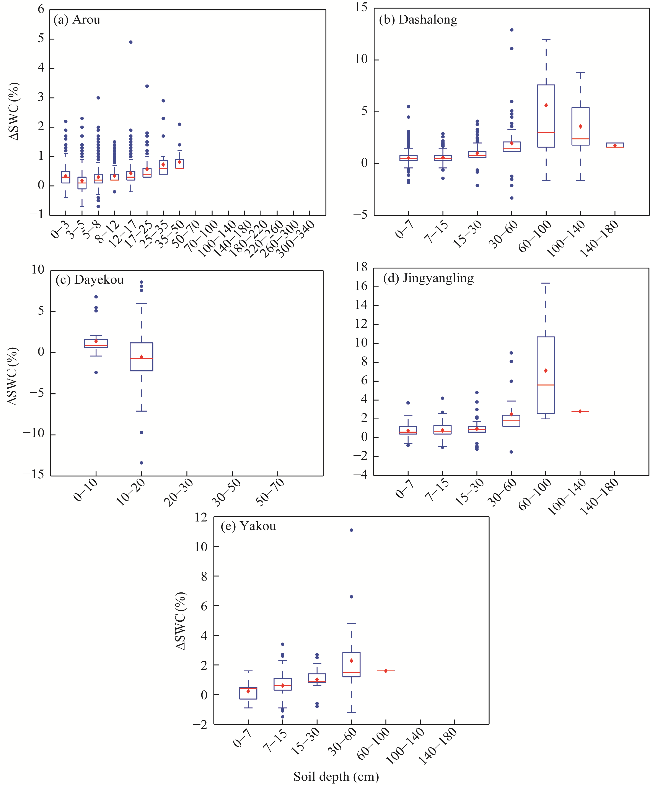
Fig. 1 Hourly changes of soil water content (ΔSWC) at five in situ observation sites. (a), Arou; (b), Dashalong; (c), Dayekou; (d), Jingyangling; (e), Yakou. Boxes in the figure indicate the IQR (interquartile range, 75th to 25th of the data). The median value is shown as a line within the box. Red diamond is shown as mean. Outlier is shown as blue circle. Whiskers extend to the most extreme value within 1.5×IQR.
Annual mean values of all components of hydrological budget during growth periods at five in situ observation sites are shown in Table 2. The highest average precipitation was recorded at Arou, followed by Dashalong, Yakou, Jingyangling, and finally Dayekou. Moreover, ET/P ratios reached their peak at grassland (Dayekou), averaging 0.9194. Subsequently, ratios decreased at alpine meadows in the following order: Arou (0.7789), Dashalong (0.6852), Jingyangling (0.3941), and Yakou (0.3384). In general, soil water storage increased at Dashalong, Jinyangling, and Yakou, while it decreased at Arou and Dayekou during growth periods (Table 2). Additionally, at Dashalong, water predominantly flows into soil pit during growth periods, as reflected by an average runoff ratio of -0.1116. Conversely, water flows out of the other sites, indicated by positive runoff ratios. The runoff ratios decreased in the following order: Yakou (0.6169), Jingyangling (0.4319), Arou (0.2463), and Dayekou (0.1493).
Table 2 Annual mean values of hydrological components during growth periods at five in situ observation sites
In situ observation site P (mm) ΔSWC (mm) ET/P ratio Runoff ratio ((Rs+RL)/P)
Arou 455.80±110.07 -11.50±25.23 0.7789 0.2463
Dashalong 302.94±51.63 129.19±81.93 0.6852 -0.1116
Dayekou 122.20±8.77 -8.40±25.88 0.9194 0.1493
Jingyangling 162.23±84.00 28.23±33.24 0.3941 0.4319
Yakou 193.42±55.96 8.64±18.24 0.3384 0.6169

Note: P, precipitation; ΔSWC, change of soil water content; ET, evapotranspiration; Rs, surface runoff, RL, lateral flow. The abbreviation are the same in the following tables and figures. Positive values of runoff ratio indicate that lateral water flows out the soil pit, and negative values of runoff ratio indicate that lateral water flows into the soil pit. Mean±SD.

3.2 Subsurface hydrological partitioning during precipitation process

As shown in Figure 2, the hourly net precipitation values decreased in the following order: Arou, Yakou, Dashalong, Jingyangling, and Dayekou. During precipitation process, ΔSWC values in the soil pits decreased in the following order: Jingyangling, Dashalong, Yakou, Dayekou, and Arou. Lateral flow values followed a decreasing trend in the order of Jingyangling, Yakou, Dashalong, Dayekou, and Arou. Because the coarser soil led to less water stored in soil and resulted in larger subsurface flows, lateral flow values were larger at loam sites (Jingyangling and Yakou) than at silt loam sites (Dayekou, Dashalong, and Arou) during precipitation process.
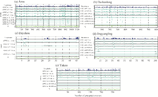
Fig. 2 Subsurface hydrological partitioning during precipitation process. (a), Arou; (b), Dashalong; (c), Dayekou; (d), Jingyangling; (e), Yakou.
Figure 2 presents the subsurface hydrological partitioning in the soil pit during precipitation process, which can be divided into three classes: class 1 (ΔSWC≥0 and RL<0), class 2 (ΔSWC<0 and RL≥0), and class 3 (ΔSWC≥0 and RL≥0). Class 1 denotes an increase in SWC caused by both precipitation and lateral flow into the soil pit. Class 2 refers to lateral flow out of the soil pit due to a combination of precipitation and a decrease in SWC. Class 3 represents the partitioning of precipitation between SWC increase and lateral flow out of soil pit. Probabilities of Class 1 ranged from 0.28 to 0.47 (Table 3), with precipitation causing a SWC increase of 26%-57%, and lateral inflow increasing SWC by 43%-74% at five observation sites. Probabilities of Class 2 ranged from 0.00 to 0.08 (Table 3), with lateral outflow ranging from 45% to 74% due to SWC decrease and from 25% to 54% due to precipitation. Probabilities of Class 3 ranged from 0.48 to 0.70 (Table 3), while 13%-35% of precipitation increased SWC, and 65%-88% contributed to lateral flow.
Table 3 Probabilities of different subsurface hydrological partitioning classes during precipitation process
In situ observation site Class 1 Class 2 Class 3
Arou 0.28 0.02 0.70
Dashalong 0.33 0.01 0.65
Dayekou 0.33 0.00 0.67
Jingyangling 0.47 0.05 0.48
Yakou 0.36 0.08 0.56

Note: Class 1 refers to ΔSWC≥0 and RL<0; Class 2 refers to ΔSWC<0 and RL≥0; and Class 3 refers to ΔSWC≥0 and RL≥0.

Figure 3a illustrates the relative importance of environmental factors for the classification of subsurface hydrological partitioning during precipitation process. The classification was primarily influenced by antecedent SWC, precipitation, and NDVI, in decreasing order of importance. The other factors had minor impacts in a decreasing order of elevation, TOC, soil texture (sand and silt), aspect, slope, and saturated hydraulic conductivity. As shown in Figure 3b-d, Class 1 generally occurred under higher precipitation and lower antecedent SWC conditions, with precipitation ranging from 0.1 to 1.5 mm/h, and saturation degree (SD) of antecedent SWC between 0.4 and 0.9. Class 2 generally occurred under lower precipitation and higher antecedent SWC conditions, with precipitation ranging from 0.1 to 0.5 mm/h, and SD of antecedent SWC between 0.6 and 0.9. On the other hand, Class 3 generally took place under medium precipitation and higher antecedent SWC conditions, with precipitation ranging from 0.1 to 0.9 mm/h, and SD of antecedent SWC between 0.5 and 0.9.
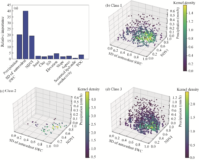
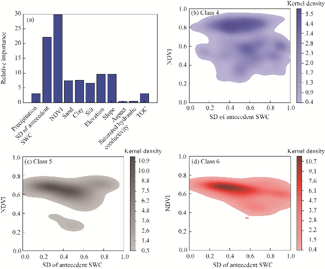
Fig. 3 Environmental factors on subsurface hydrological partitioning classes during precipitation process. (a), relative importance; (b), Class 1; (c), Class 2; (d), Class 3. SD, saturation degree; NDVI, normalized difference vegetation index; TOC, total organic carbon.
Furthermore, Class 2 exclusively occurred in alpine meadows. For Class 2, the probability was 1.00, which the decrease of SWC occurred in 0-17 cm soil depth at Arou, while the probabilities were 1.00, 1.00, and 0.95, which the decrease of SWC occurred in 0-30 cm soil depth at Dashalong, Jingyangling, and Yakou, respectively. Additionally, average antecedent SWC values in decreasing soil depths were generally higher than the corresponding field capacities at four alpine meadows as shown in Table 1 Meanwhile, in deep soil depths, average antecedent SWC values were lower than field capacities.
In summary, lateral flow significantly influenced subsurface hydrological partitioning during precipitation process. The most common partitioning class (Class 3) was the increase of SWC and lateral flow out of the soil pit, with 65%-88% precipitation contributing to lateral flow. The second common partitioning class (Class 1) showed an increase in SWC caused by both precipitation and lateral flow into the soil pit, with lateral flow contributing to SWC increase ranging from 43% to 74%, which was notably larger than SWC increase caused by precipitation. There was also a minor possibility of lateral flow out of the soil pit due to a combination of precipitation and decrease of SWC (Class 2), which occurred only in alpine meadows. In this case, lateral flow, instead of vertical flow, occurred when shallow soil was wetter than field capacity and deep soil was still below field capacity.

3.3 Subsurface hydrological partitioning during ET process

As shown in Figure 4, the hourly ET values decreased in the following order: Arou, Dashalong, Yakou, Dayekou, and Jingyangling. During ET process, ΔSWC value in the soil pits was -0.13 (±1.47) mm/h, and absolute lateral flow value was 0.65 (±1.32) mm/h at Dayekou. At the other in situ observation sites, average ΔSWC values ranged from -0.01 to 0.08 mm/h. Average absolute lateral flow values ranged from 0.21 to 0.32 mm/h. It was observed that both soil water dynamics and lateral flow during ET process exhibited higher average value on grassland than on alpine meadows, with extremely small variations in SWC observed on alpine meadows.
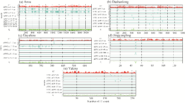
Fig. 4 Subsurface hydrological partitioning during evapotranspiration (ET) process. (a), Arou; (b), Dashalong; (c), Dayekou; (d), Jingyangling; (e), Yakou.
As shown in Figure 4, the subsurface hydrological partitioning during ET process can be divided into three classes: Class 4 (ΔSWC≤0 and RL≤0), Class 5 (ΔSWC>0 and RL≤0), and Class 6 (ΔSWC≤0 and RL>0). Class 4 refers to the situation where ET is provided by SWC decrease and lateral flow into the soil pit. Class 5 refers to the situation where both ET and SWC increases are provided by lateral flow into the soil pit. Class 6 refers to the situation where SWC decrease in the soil pit is attributed to a combination of ET and lateral flow out of the soil pit. Significant differences in the classification of subsurface hydrological partitioning were observed among different vegetation types during ET process. On alpine meadows, Class 4 was the primary hydrological partitioning class with probabilities ranging from 0.96 to 1.00 (Table 4). It was noted that 98%-100% of ET provided by lateral flow for Class 4 on alpine meadows. In the case of grassland at Dayekou, Class 4 predominated with a probability of 0.78 (Table 4), and 100% of ET was provided by lateral flow, evidenced by all ΔSWC values being zero. Class 5 was the least common class with a probability of 0.09 (Table 4), where 5%-35% of lateral flow contributed to ET and 65%-95% of lateral flow contributed to an increase in SWC. Class 6 occurred with a probability of 0.12 (Table 4), and 84% of the decrease in SWC was attributed to lateral flow out of the soil pit. These findings underscored the complex subsurface hydrological dynamics and highlighted the pivotal role of lateral flow during ET process.
Table 4 Probabilities of different subsurface hydrological partitioning classes during ET process
In situ observation site Class 4 Class 5 Class 6
Arou 1.00 0.00 0.00
Dashalong 0.97 0.00 0.02
Dayekou 0.78 0.09 0.12
Jingyangling 0.99 0.01 0.00
Yakou 0.96 0.01 0.03

Note: Class 4 refers to ΔSWC≤0 and RL≤0; Class 5 refers to ΔSWC>0 and RL≤0; and Class 6 refers to ΔSWC≤0 and RL>0.

Figure 5a shows the relative importance of different environmental factors for subsurface hydrological partitioning classes during ET process. Classification was mainly influenced by NDVI and antecedent SWC. The other factors displayed minor impacts in a decreasing order of elevation, slope, soil texture (clay, sand, and silt), TOC, ET, saturated hydraulic conductivity, and aspect. As shown in Figure 5b-d, Class 4 generally occurred under higher NDVI (0.6-0. 9) and higher antecedent SWC (SD: 0.3-0.9) conditions. Class 5 occurred under lower NDVI (0.6-0.7) and lower antecedent SWC (SD: 0.1-0.6) conditions. Class 6 generally occurred under lower NDVI (0.6-0.7) and medium antecedent SWC (SD: 0.2-0.7) conditions.
Fig. 5 Environmental factors on subsurface hydrological partitioning classes during ET process. (a), relative importance; (b), Class 4; (b), Class 5; (d), Class 6.
In summary, during ET process, both soil water dynamics and lateral flow exhibited larger variations on grassland than on alpine meadows. Significant differences in the classification of subsurface hydrological partitioning were observed among different vegetation types during ET process. On alpine meadows, the majority of responses involved ET provided by SWC decrease and lateral flow into the soil pit (Class 4), with lateral flow contributing to 98%-100% of ET. Conversely, on grassland, there was a probability of 0.12, which ET was entirely provided by SWC decrease (Class 6). In this case, there was a high probability (0.98) that soil water responses only occurred at 10-20 cm depth. Furthermore, there was a high probability of 0.87, which ET was entirely provided by lateral flow (Classes 4 and 5). Classification of subsurface hydrological partitioning during ET process was primarily determined by NDVI and antecedent SWC, rather than ET itself.

3.4 RF model in simulating lateral flow

In this study, RF model was established separately to estimate lateral flow during precipitation and ET processes. Due to limited data availability on grassland during precipitation process, RF model for estimating lateral flow during precipitation process was only established at four alpine meadow observation sites. As shown in Figure 6a-d, for the training dataset, r values of RF model ranged from 0.841 to 0.943, while RMSE values ranged from 0.30 to 1.16 mm/h at four alpine meadow sites. For the test dataset, r values of RF model ranged from 0.723 to 0.954, while RMSE values ranged from 0.27 to 3.50 mm/h at the same sites. The results indicated that the established RF model for estimating lateral flow during precipitation process performed well in the study area.
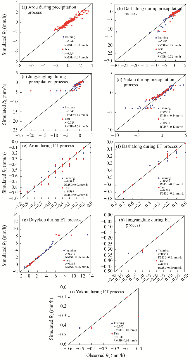
Fig. 6 Simulated result of lateral flow through random forest model. (a-d), Arou, Dashalong, Jingyangling, and Yakou sites during precipitation process; (e-i), Arou, Dashalong, Dayekou, Jingyangling, and Yakou sites during ET process. RMSE, root mean square errors.
During ET process, RF model for estimating lateral flow was established at five in situ observation sites. For the training dataset, r values of RF model ranged from 0.977 to 0.999, while RMSE values ranged from 0.01 to 0.26 mm/h (Fig. 6e-i). For the test dataset, r values of RF models ranged from 0.944 to 0.998, while RMSE values ranged from 0.01 to 0.26 mm/h. The results indicated that the established RF models in estimating lateral flow during ET process also showed excellent performance.

3.5 Performance of CLM through bias correction

During precipitation process, profile ΔSWC simulated by CLM was bias corrected using simulated lateral flow from RF model at four alpine meadow observation sites. The bias-corrected ΔSWC values showed large improvements, with increased r values ranging from 0.177 to 0.853 and decreased RMSE values ranging from -0.13 to 1.21 mm/h (Fig. 7a-d). However, the bias-corrected CLM simulations still performed worse for extreme values. The bias-corrected ET values showed large improvements, with increased r values ranging from 0.338 to 0.905 and decreased RMSE values ranging from 0.04 and 0.20 mm/h (Fig. 7e-i).
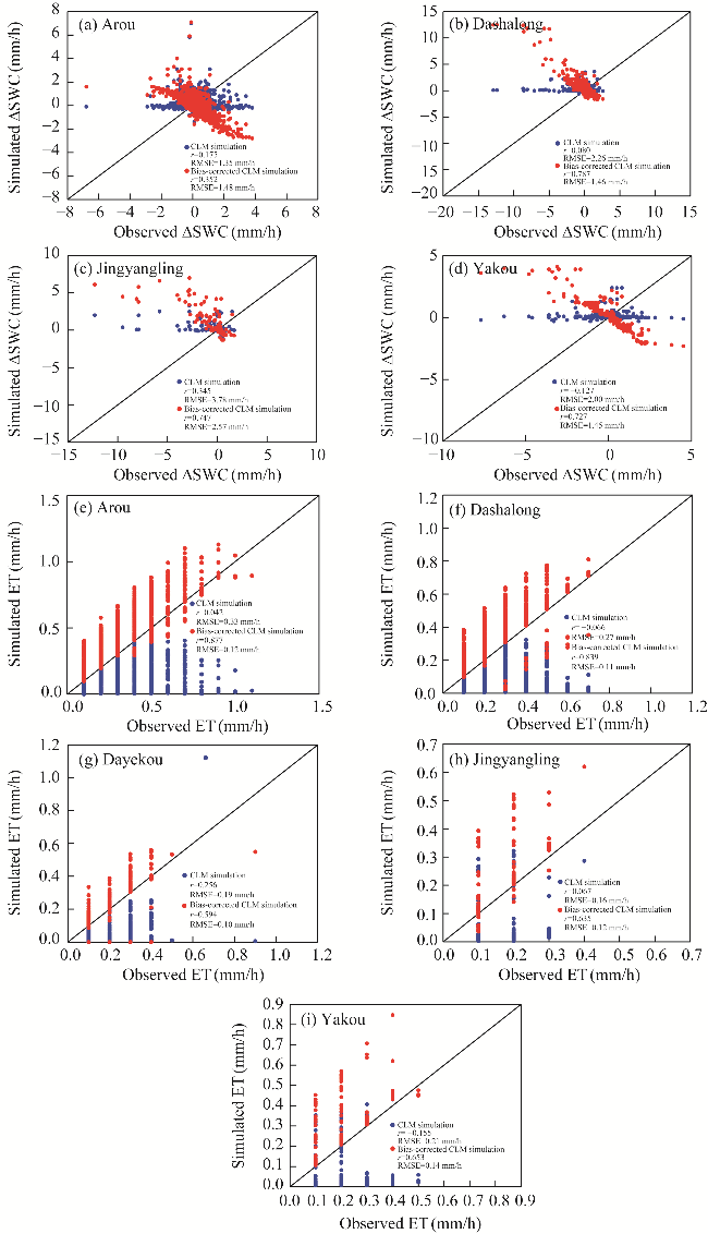
Fig. 7 Simulated results of ΔSWC and ET by CLM and bias corrected CLM. (a-d), ΔSWC at Arou, Dashalong, Jingyangling, and Yakou sites during precipitation process; (e-i), ET at Arou, Dashalong, Dayekou, Jingyangling, and Yakou during ET process. CLM, community land model.
This study highlighted the importance of lateral flow in subsurface hydrological partitioning during both precipitation and ET processes. Furthermore, the bias corrected CLM simulation demonstrated large improvements in estimating both ΔSWC and ET under both processes. Therefore, the findings of this study suggested the necessity of developing three-dimensional ESMs that incorporated lateral flow in mountainous area, rather than solely focusing on adjusting model parameterization scheme or model parameters.

4 Discussion

4.1 Impacts of topography on hydrological partitioning during growth periods

In the HRB, there is a notable vertical zonality (He et al., 2009). Additionally, above 3600 m, the main runoff generation area of the HRB generates approximately 83% of the total runoff for the entire basin (Kang et al., 2008; Chen et al., 2014). Therefore, this study examined the impacts of topographic features on hydrological partitioning above and below 3600 m.
Combined with previous research, ET/P ratios decreased with elevation during growth periods (Kang et al., 2008; Chen et al., 2014; Yang et al., 2019). This result indicated that less precipitation was returned to the atmosphere through ET at higher elevations compared with lower elevations due to lower transpiration rates caused by lower temperatures at higher elevations (Mujawamariya et al., 2018). Furthermore, runoff ratios generally increased with increasing elevation in the study area. It is generally considered that average runoff ratios are 0.4600 above 3600 m and 0.1800 below 3600 m in the HRB (Kang et al., 2008; Chen et al., 2014). Interestingly, although Dashalong was located in the runoff generation area with elevation above 3600 m, it had an average runoff ratio of 0.1116 in this study. The low runoff ratio can be attributed the reason that the site has a slope of 0° and is surrounded by higher elevation, creating a depression that causes water flow into the site (Fan et al., 2019). Therefore, the hydrological partitioning at point scale is significantly influenced by topographic features, indicating the need of small-scale investigation and simulation in high mountainous area.
During growth periods, it was generally observed that SWC increased at Dashalong, Jinyangling, and Yakou. While at Arou and Dayekou, there was a decrease in SWC. In the upper reaches of the HRB, the change of soil water storage during growth periods was influenced not only by precipitation and ET, but also by the antecedent thawed soil water and melted snow (Tong et al., 2018). Due to soil thawing and snow melting, soil water rapidly increased during March-May before growth periods (Tong et al., 2018). Thus, soil water was replenished during March-May and consumed by ET during growth periods at Arou and Dayekou below 3600 m. However, at Dashalong, Jingyangling, and Yakou above 3600 m, soil water was still replenished by precipitation during growth periods, which resulted in higher SWC at higher elevation in the study area (Zhao et al., 2014).

4.2 Impacts of environmental factors on subsurface hydrological partitioning during precipitation process

Antecedent SWC is the most important factor influencing hydrological partitioning classes in subsurface during precipitation process. As shown in Figure 8, lateral flows observed at Dayekou and Jingyangling exhibited a pattern that tended to flow out of the soil pit, especially when the antecedent SWC was lower in shallow soil (0-20 cm at Dayekou and 0-60 cm at Jingyangling) while being higher in deeper soil. This phenomenon is attributed to the dominance of vertical preferential flow on hillslopes with well-drained and highly porous soils (Grayson et al., 1997; Jarecke et al., 2021). The slope gradient and soil texture also contribute to this phenomenon, as seen at Jingyangling where the slope is 12° and the soil texture is loam, leading to the domination of vertical preferential flow in 0-60 cm shallow soil depth. The presence of dense roots can further enhance this phenomenon, creating well-drained and highly porous soils (Beven and Germann, 1982; Liu and Lin, 2015; Wiekenkamp et al., 2016). With soil texture of silt loam, the root of grass is mainly distributed in 0-20 cm soil depth at Dayekou (Gao, 2020). Therefore, vertical preferential flow occurred in well-drained and highly porous soils that dominated by vegetation roots in 0-20 cm soil depth at Dayekou. Therefore, lateral flow tends to occur on the soil interface between well-drained and highly porous soils.
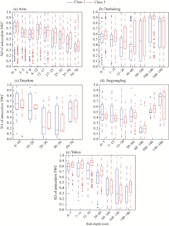
Fig. 8 SD of antecedent SWC for two subsurface hydrological partitioning classes (Class 1 and Class 3) during precipitation process. (a), Arou; (b), Dashalong; (c), Dayekou; (d), Jingyangling; (e), Yakou. Boxes in the figure indicate the IQR (interquartile range, 75th to 25th of the data). The median value is shown as a line within the box. Outlier is shown as blue or red circle. Whiskers extend to the most extreme value within 1.5×IQR.
Conversely, lateral flows tended to flow out of the soil pit under higher antecedent SWC in soil profiles at Arou and Dashalong, and under higher antecedent SWC throughout the soil profile except for 60-140 cm depth at Yakou (Fig. 8). The slope is 2° at Arou, 0° at Dashalong, and 4° at Yakou (Table 1). The relatively flatter terrain at these sites promotes easier saturation of wetter soil, leading to subsurface flows (Hardie et al., 2012; Hardie et al., 2013). In summary, the impact of antecedent SWC on subsurface hydrological partitioning classes during precipitation process varied based on the specific combinations of hillslope position, vegetation root distribution, and soil texture. This result highlighted further investigation of subsurface flows under different environmental conditions on hillslope scale.
It should be noted that on alpine meadows, lateral flow, rather than vertical flow, occurred when shallow soil was wetter than field capacity, while deeper soil remained below field capacity. Previous studies have highlighted the interaction between vertical and lateral soil water transport in mountainous areas, and emphasized that this phenomenon takes place between different soil depths (He et al., 2009; Lee and Kim, 2022). However, in ESMs, lateral flow was generally simulated between soil profiles when entire soil profile was saturated, rather than between individual soil depths. This result necessitates the three-dimensional simulation between soil depths in ESMs.

4.3 Impacts of vegetation roots on subsurface hydrological partitioning during ET process

During ET process, vegetation primarily influences the subsurface hydrological cycle by root water uptake (Fan et al., 2019; Zhang et al., 2021). Larger ΔSWC values were observed on grassland, with minimal SWC variations on alpine meadows during ET process. Moreover, lateral flow also exhibited higher average value and standard deviations on grassland compared to alpine meadows. The result indicated that root water uptake caused larger variations in the subsurface hydrological cycle on grassland than on alpine meadows. In the upper reaches of the HRB, a substantial portion (more than 90%) of root lengths in alpine meadows is concentrated within 0-10 cm, and around 90% of the roots are fine roots less than 0.5 mm in diameter (Huang et al., 2011; Fan et al., 2020). The entanglement of fine roots in the surface soil (0-10 cm) suggested that alpine meadows tended to utilize non-local water through lateral root systems (Fan et al., 2020), resulting in minimal SWC variations. Thus, almost all ET (98%-100%) was facilitated by lateral root water uptake in 0-10 cm soil depth, and SWC in the soil pit displayed minimal fluctuation.
Furthermore, on grassland, the majority of responses involved ET provided by SWC decrease and lateral flow into the soil pit (Class 4). In this scenario, there was a 0.78 probability that all ET was supplied through lateral flow without SWC variations. Since ET is the sum of plant transpiration and soil evaporation in this study, the absence of SWC variations suggested that ET solely depended on plant transpiration. Therefore, almost all the transpiration was provided by lateral root water uptake on alpine meadows, and there was a high probability of 0.78, confirming that all transpiration was provided by lateral flow on grassland. Previous research has found that plant water use is much larger than that estimated from soil water dynamics by both observation and model simulation (Dawson and Ehleringer, 1991; Lee et al., 2005; Yaseef et al., 2009; Hu et al., 2010). Therefore, the primary reason for the underestimation of plant transpiration derived from soil water dynamics is the neglect of lateral root water uptake. This finding highlights the necessity for a more comprehensive and large-scale examination of CZ structure to accurately predict multiple sources of plant-available water (Brooks et al., 2009).
Additionally, there was a 0.12 probability (Class 6) on grassland where ET was entirely provided by SWC decrease. In this case, SWC variations typically occurred within 10-20 cm soil depth. This result can be attributed to the aggregation of grass roots in 0-20 cm soil depth in the Qilian Mountains (Gao, 2020). Grasses often utilize their deep roots for water uptake during ET process (Li et al., 2021; Miguez-Macho and Fan, 2021), resulting in more pronounced variations in SWC near root zone, while variations in the intermediate and peripheral areas are generally less significant (Zhang et al., 2021). Moreover, water uptake through deep roots of both trees and grasses during ET process (Li et al., 2021; Miguez-Macho and Fan, 2021) highlights the correlation between transpiration rate and subsurface water storage, rather than surface water supply on the hillslope scale (Tromp-van Meerveld and McDonnell, 2006; Yaseef et al., 2009).

4.4 Limitation

Firstly, although the observed SWC data have been quality-controlled, their precision is currently limited to ±0.003 m3/m3 (Bai et al., 2020). Meanwhile, ET data used in this study were observed by eddy covariance measurements, which provided data at larger spatial scales compared with the point-scale SWC observation (Yaseef et al., 2009). This disparity in observation accuracy and scale introduces uncertainty in estimating ΔSWC due to potential observational errors. To mitigate the impacts of measurement errors in SWC, we considered only absolute ΔSWC values larger than 0.003 m3/m3 in this study (Lozano-Parra et al., 2015, 2016). ET datasets have been rigorously quality controlled, and five in situ observation sites are characterized by relatively uniform vegetation types. Therefore, the uncertainty associated with ΔSWC and ET was minimized to the best extent possible using monitoring instrument and methods available. However, it should be noted that discarding SWC variations less than 0.003 m3/m3 may lead to overestimation of runoff lateral flow during precipitation and underestimation during ET. Secondly, it is worth mentioning that analysis of lateral flow in this study was conducted at hourly intervals. However, this approach overlooks any lateral flows that occur more frequently than sampling frequency (Goodwell et al., 2020). Investigation into these finer temporal scales will be addressed in future research.

5 Conclusions

Flux quantification, especially subsurface hydrological partitioning is a major challenge in CZ. This study applied a comprehensive investigation of three-dimensional subsurface hydrological partitioning in an alpine mountainous area, northwestern China through establishing RF model to simulate lateral flow and correcting simulation.
In the upper reaches of the HRB, lateral flow played a significant role in subsurface hydrological partitioning. During precipitation process, lateral flow accounted for the majority when precipitation increased SWC and lateral flow from the soil pit. Notably, when SWC increased by lateral flow in the soil pit and precipitation, the contribution of lateral flow exceeded that of precipitation. On alpine meadows, lateral flow from the soil pit occurred when shallow soil was wetter than field capacity and the deep soil remained below field capacity. Furthermore, neglecting lateral root water uptake is the main reason for underestimation of plant transpiration from soil water dynamics based on water balance equation. RF model developed in this study effectively simulated lateral flow under both precipitation and ET processes, resulting in substantial improvements in CLM simulation. In conclusion, integrating lateral flow dynamics in ESMs is crucial for improving hydrological modeling in alpine mountainous areas.

Conflict of interest

The authors declare that they have no known competing financial interests or personal relationships that could have appeared to influence the work reported in this paper.

Acknowledgements

The study was funded by the National Natural Science Foundation of China (42371022, 42030501, 41877148).

Author contributions

Conceptualization: ZHANG Lanhui; Methodology: ZHANG Lanhui, TU Jiahao, AN Qi; Formal analysis: LIU Yu, XU Jiaxin, ZHANG Haixin; Writing - original draft preparation: ZHANG Lanhui, TU Jiahao; Writing - review and editing: ZHANG Lanhui, TU Jiahao, AN Qi, LIU Yu, XU Jiaxin, ZHANG Haixin; Funding acquisition: ZHANG Lanhui. All authors approved the manuscript.
Open Access This article is licensed under a Creative Commons Attribution 4.0 International License, which permits use, sharing, adaptation, distribution and reproduction in any medium or format, as long as you give appropriate credit to the original author(s) and the source, provide a link to the Creative Commons licence, and indicate if changes were made. The images or other third party material in this article are included in the article's Creative Commons licence, unless indicated otherwise in a credit line to the material. If material is not included in the article's Creative Commons licence and your intended use is not permitted by statutory regulation or exceeds the permitted use, you will need to obtain permission directly from the copyright holder. To view a copy of this licence, visit http://creativecommons.org/licenses/by/4.0/.
[1]
Bai X, Zhang L H, He C S, et al. 2020. Estimating regional soil moisture distribution based on NDVI and land surface temperature time series data in the upstream of the Heihe River Watershed, Northwest China. Remote Sensing, 12(15): 2414, doi: 10.3390/rs12152414.

[2]
Beven K, Germann P. 1982. Macropores and water flow in soils. Water Resources Research, 18(5): 1311-1325.

[3]
Brantley S L, Goldhaber M B, Ragnarsdottir K V. 2007. Crossing disciplines and scales to understand the critical zone. Elements, 3(5): 307-314.

[4]
Breiman L. 2001. Random forests. Machine Learning, 45: 5-32.

[5]
Brooks J R, Barnard H R, Coulombe R, et al. 2009. Ecohydrologic separation of water between trees and streams in a Mediterranean climate. Nature Geoscience, 3(2): 100-104.

[6]
Chen R S, Yang Y, Han C T, et al. 2014. Field experimental research on hydrological function over several typical underlying surfaces in the cold regions of western China. Advances in Earth Science, 29(4): 507-514. (in Chinese)

[7]
Dawson T E, Ehleringer J R. 1991. Streamside trees that do not use stream water. Nature, 350: 335-337.

[8]
Fan B, Lin L, Cao G M, et al. 2020. Relationship between plant roots and physical soil properties in alpine meadows at different degradation stages. Acta Ecologica Sinica, 40(7): 2300-2309. (in Chinese)

[9]
Fan Y. 2015. Groundwater in the Earth's critical zone: Relevance to large-scale patterns and processes. Water Resources Research, 51(5): 3052-3069.

[10]
Fan Y, Clark M, Lawrence D M, et al. 2019. Hillslope hydrology in global change research and earth system modeling. Water Resources Research, 55(2): 1737-1772.

[11]
Gao Y. 2020. Evapotranspiration and water balance of subalpine meadows in the Qilian Mountains. PhD Thesis. Lanzhou: Lanzhou University. (in Chinese)

[12]
Goodwell A E, Jiang P, Ruddell B L, et al. 2020. Debates-does information theory provide a new paradigm for Earth science? Causality, interaction, and feedback. Water Resources Research, 56(2): e2019WR024940, doi: 10.1029/2019wr024940.

[13]
Grant G E, Dietrich W E. 2017. The frontier beneath our feet. Water Resources Research, 53(4): 2605-2609.

[14]
Grayson R B, Western A W, Chiew F H S, et al. 1997. Preferred states in spatial soil moisture patterns: Local and nonlocal controls. Water Resources Research, 33(12): 2897-2908.

[15]
Grömping U. 2009. Variable importance assessment in regression: Linear regression versus random forest. The American Statistician, 63(4): 308-319.

[16]
Guo L, Lin H. 2016. Critical zone research and observatories: Current status and future perspectives. Vadose Zone Journal, 15(9): 1-14.

[17]
Han X T, Liu J T, Srivastava P, et al. 2021. The dominant control of relief on soil water content distribution during wet-dry transitions in headwaters. Water Resources Research, 57(11): e2021WR029587, doi: 10.1029/2021wr029587.

[18]
Hardie M A, Doyle R B, Cotching W E, et al. 2012. Influence of antecedent soil moisture on hydraulic conductivity in a series of texture-contrast soils. Hydrological Processes, 26(20): 3079-3091.

[19]
Hardie M A, Lisson S, Doyle R, et al. 2013. Determining the frequency, depth and velocity of preferential flow by high frequency soil moisture monitoring. Journal of Contaminant Hydrology, 144(1): 66-77.

[20]
He C S, Demarchi C, Ecroley T, et al. 2009. Hydrologic modeling of the Heihe watershed by DLBRM in Northwest China. Journal of Glaciology and Geocryology, 31(3): 410-421. (in Chinese)

[21]
He Z, Zhao W, Liu H, et al. 2012. Effect of forest on annual water yield in the mountains of an arid inland river basin: A case study in the Pailugou catchment on northwestern China's Qilian Mountains. Hydrological Processes, 26(4): 613-621.

[22]
Hu G R, Li X Y, Yang X F, et al. 2022. Identifying spatiotemporal patterns of hillslope subsurface flow in an alpine critical zone on the Qinghai-Tibetan Plateau based on three-year, high-resolution field observations. Water Resources Research, 58(11): e2022WR032098, doi: 10.1029/2022wr032098.

[23]
Hu J, Moore D J, Burns S P, et al. 2010. Longer growing seasons lead to less carbon sequestration by a subalpine forest. Global Change Biology, 16(2): 771-783.

[24]
Huang D Q, Yu L, Zhang Y S, et al. 2011. Belowground biomass and its relationship to environmental factors of natural grassland on the northern slopes of the Qilian Mountains. Acta Prataculturae Sinica, 20(5): 1-10. (in Chinese)

[25]
Jarecke K M, Bladon K D, Wondzell S M. 2021. The influence of local and nonlocal factors on soil water content in a steep forested catchment. Water Resources Research, 57(5): e2020WR028343, doi: 10.1029/2020wr028343.

[26]
Kang E S, Chen R S, Zhang Z H, et al. 2008. Some problems facing hydrological and ecological researches in the mountain watershed at the upper stream of an inland river basin. Advances in Earth Science, 23(7): 675-681. (in Chinese)

[27]
Kushwaha A P, Tiwari A D, Dangar S, et al. 2021. Multimodel assessment of water budget in Indian sub-continental river basins. Journal of Hydrology, 603: 126977, doi: 10.1016/j.jhydrol.2021.126977.

[28]
Lawrence D M, Fisher R A, Koven C D, et al. 2019. The community land model version 5: Description of new features, benchmarking, and impact of forcing uncertainty. Journal of Advances in Modeling Earth Systems, 11(12): 4245-4287.

[29]
Lee E, Kim S. 2022. Spatiotemporal soil moisture response and controlling factors along a hillslope. Journal of Hydrology, 605: 127382, doi: 10.1016/j.jhydrol.2021.127382.

[30]
Lee J E, Oliveira R S, Dawson T E, et al. 2005. Root functioning modifies seasonal climate. Proceedings of the National Academy of Sciences of the United States of America, 102(49): 17576-17581.

[31]
Li W T, Migliavacca M, Forkel M, et al. 2021. Revisiting global vegetation controls using multilayer soil moisture. Geophysical Research Letters, 48(11): e2021GL092856, doi: 10.1029/2021gl092856.

[32]
Li X, Cheng G D, Fu B J, et al. 2022. Linking critical zone with watershed science: The example of the Heihe River Basin. Earth's Future, 10(11): e2022EF002966, doi: 10.1029/2022ef002966.

[33]
Li Z L, Xu Z X, Shao Q X, et al. 2009. Parameter estimation and uncertainty analysis of SWAT model in upper reaches of the Heihe River Basin. Hydrological Processes, 23(19): 2744-2753.

[34]
Liaw A, Wiener M. 2002. Classification and regression by random forest. R News, 2(3): 18-22.

[35]
Lin H. 2010. Earth's critical zone and hydropedology: Concepts, characteristics, and advances. Hydrology and Earth System Sciences, 14(1): 25-45.

[36]
Liu H, Lin H. 2015. Frequency and control of subsurface preferential flow: From pedon to catchment scales. Soil Science Society of America Journal, 79(2): 362-377.

[37]
Liu Z, Hou H, Zhang L, et al. 2022. Event-based bias correction of the GPM IMERG V06 product by random forest method over Mainland China. Remote Sensing, 14: 3859, doi: 10.3390/rs14163859.

[38]
Lozano-Parra J, Schnabel S, Ceballos-Barbancho A. 2015. The role of vegetation covers on soil wetting processes at rainfall event scale in scattered tree woodland of Mediterranean climate. Journal of Hydrology, 529: 951-961.

[39]
Lozano-Parra J, van Schaik N L M B, Schnabel S, et al. 2016. Soil moisture dynamics at high temporal resolution in a semi-arid Mediterranean watershed with scattered tree cover. Hydrological Processes, 30(8): 1155-1170.

[40]
Miguez-Macho G, Fan Y. 2021. Spatiotemporal origin of soil water taken up by vegetation. Nature, 598(7882): 624-628.

[41]
Moriasi D N, Arnold J G, Van Liew M W, et al. 2007. Model evaluation guidelines for systematic quantification of accuracy in watershed simulation. Transactions of the Asabe, 50(3): 885-900.

[42]
Mu Y M, Yuan Y, Jia X, et al. 2022. Hydrological losses and soil moisture carryover affected the relationship between evapotranspiration and rainfall in a temperate semi-arid shrubland. Agricultural and Forest Meteorology, 315: 108831, doi: 10.1016/j.agrformet.2022.108831.

[43]
Mujawamariya M, Manishimwe A, Ntirugulirwa B, et al. 2018. Climate sensitivity of tropical trees along an elevation gradient in Rwanda. Forests, 9(10): 647, doi: 10.3390/f9100647.

[44]
Parsekian A D, Singha K, Minsley B J, et al. 2015. Multiscale geophysical imaging of the critical zone. Reviews of Geophysics, 53(1): 1-26.

[45]
Peterson A M, Helgason W H, Ireson A M. 2019. How spatial patterns of soil moisture dynamics can explain field-scale soil moisture variability: Observations from a sodic landscape. Water Resources Research, 55(5): 4410-4426.

[46]
Rahmati O, Pourghasemi H R, Melesse A M. 2016. Application of GIS-based data driven random forest and maximum entropy models for groundwater potential mapping: A case study at Mehran Region, Iran. Catena, 137: 360-372.

[47]
Rasmussen C, Pelletier J D, Troch P A, et al. 2015. Quantifying topographic and vegetation effects on the transfer of energy and mass to the critical zone. Vadose Zone Journal, 14(11): 1-16.

[48]
Richter D deB, Mobley M L. 2009. Monitoring Earth's critical zone. Science, 326(5956): 1067-1068.

[49]
Tian J, Zhang B Q, He C S, et al. 2017. Variability in soil hydraulic conductivity and soil hydrological response under different land covers in the mountainous area of the Heihe River Watershed, Northwest China. Land Degradation & Development, 28(4): 1437-1449.

[50]
Tian J, Zhang B Q, He C S, et al. 2019. Dynamic response patterns of profile soil moisture wetting events under different land covers in the Mountainous area of the Heihe River Watershed, Northwest China. Agricultural and Forest Meteorology, 271: 225-239.

[51]
Tong Y Q, Wang P, Li X Y, et al. 2018. Water budget and evapotranspiration partition in an alpine meadow ecosystem in the upstream of the Heihe River, China. Acta Ecologica Sinica, 38(20): 7400-7411. (in Chinese)

[52]
Tromp-van Meerveld H J, McDonnell J J. 2006. On the interrelations between topography, soil depth, soil moisture, transpiration rates and species distribution at the hillslope scale. Advances in Water Resources, 29(2): 293-310.

[53]
Vereecken H, Huisman J A, Hendricks Franssen H J, et al. 2015. Soil hydrology: Recent methodological advances, challenges, and perspectives. Water Resources Research, 51(4): 2616-2633.

[54]
Vereecken H, Amelung W, Bauke S L, et al. 2022. Soil hydrology in the Earth system. Nature Reviews Earth & Environment, 3(9): 573-587.

[55]
Wei S G, Dai Y J, Liu B Y, et al. 2013. A China data set of soil properties for land surface modeling. Journal of Advances in Modeling Earth Systems, 5(2): 212-224.

[56]
Wiekenkamp I, Huisman J A, Bogena H R, et al. 2016. Spatial and temporal occurrence of preferential flow in a forested headwater catchment. Journal of Hydrology, 534: 139-149.

[57]
Wlostowski A N, Molotch N, Anderson S P, et al. 2021. Signatures of hydrologic function across the critical zone observatory network. Water Resources Research, 57(3): e2019WR026635, doi: 10.1029/2019wr026635.

[58]
Xu S. 2022. Estimation of evapotranspiration under soil water stress in arid and semi-arid areas. MSc Thesis. Lanzhou: Lanzhou University. (in Chinese)

[59]
Yang C Y, Huang Y M, Li E G, et al. 2019. Rainfall interception of typical ecosystems in the Heihe River Basin: Based on high temporal resolution soil moisture data. Journal of Geographical Sciences, 29(9): 1527-1547.

[60]
Yaseef N R, Yakir D, Rotenberg E, et al. 2009. Ecohydrology of a semi-arid forest: Partitioning among water balance components and its implications for predicted precipitation changes. Ecohydrology, 3(2): 143-154.

[61]
Zeng Z Z, Peng L Q, Piao S L. 2018. Response of terrestrial evapotranspiration to Earth's greening. Current Opinion in Environmental Sustainability, 33: 9-25.

[62]
Zhang J, Li Y, Yang T Q, et al. 2021. Spatiotemporal variation of moisture in rooted-soil. Catena, 200: 105736, doi: 10.1016/j.catena.2021.105736.

[63]
Zhang L H, Jin X, He C S, et al. 2016. Comparison of SWAT and DLBRM for hydrological modeling of a mountainous watershed in arid northwest China. Journal of Hydrologic Engineering, 21(5): 04016007, doi: 10.1061/(asce)he.1943-5584.0001313.

[64]
Zhang L H, He C S, Zhang M M, et al. 2019. Evaluation of the SMOS and SMAP soil moisture products under different vegetation types against two sparse in situ networks over arid mountainous watersheds, Northwest China. Science China Earth Sciences, 62(4): 703-718.

[65]
Zhang L H, Ning F W, Bai X L, et al. 2023. Performance evaluation of CLM5.0 in simulating liquid soil water in high mountainous area, Northwest China. Journal of Mountain Science, 20(7): 1865-1883.

[66]
Zhang N, Quiring S, Ochsner T, et al. 2017. Comparison of three methods for vertical extrapolation of soil moisture in Oklahoma. Vadose Zone Journal, 16(10): 1-19.

[67]
Zhao C, Zhang L H, Li J L, et al. 2014. Analysis of the relationships between the spatial variations of soil moisture and the environmental factors in the upstream of the Heihe River watershed. Journal of Lanzhou University (Natural Sciences), 50(3): 338-347. (in Chinese)

文章导航

/