
Three-dimensional (3D) parametric measurements of individual gravels in the Gobi region using point cloud technique
Received date: 2023-12-11
Revised date: 2024-03-09
Accepted date: 2024-03-12
Online published: 2024-04-30
JING Xiangyu , HUANG Weiyi , KAN Jiangming . [J]. Journal of Arid Land, 2024 , 16(4) : 500 -517 . DOI: 10.1007/s40333-024-0073-4
Gobi spans a large area of China, surpassing the combined expanse of mobile dunes and semi-fixed dunes. Its presence significantly influences the movement of sand and dust. However, the complex origins and diverse materials constituting the Gobi result in notable differences in saltation processes across various Gobi surfaces. It is challenging to describe these processes according to a uniform morphology. Therefore, it becomes imperative to articulate surface characteristics through parameters such as the three-dimensional (3D) size and shape of gravel. Collecting morphology information for Gobi gravels is essential for studying its genesis and sand saltation. To enhance the efficiency and information yield of gravel parameter measurements, this study conducted field experiments in the Gobi region across Dunhuang City, Guazhou County, and Yumen City (administrated by Jiuquan City), Gansu Province, China in March 2023. A research framework and methodology for measuring 3D parameters of gravel using point cloud were developed, alongside improved calculation formulas for 3D parameters including gravel grain size, volume, flatness, roundness, sphericity, and equivalent grain size. Leveraging multi-view geometry technology for 3D reconstruction allowed for establishing an optimal data acquisition scheme characterized by high point cloud reconstruction efficiency and clear quality. Additionally, the proposed methodology incorporated point cloud clustering, segmentation, and filtering techniques to isolate individual gravel point clouds. Advanced point cloud algorithms, including the Oriented Bounding Box (OBB), point cloud slicing method, and point cloud triangulation, were then deployed to calculate the 3D parameters of individual gravels. These systematic processes allow precise and detailed characterization of individual gravels. For gravel grain size and volume, the correlation coefficients between point cloud and manual measurements all exceeded 0.9000, confirming the feasibility of the proposed methodology for measuring 3D parameters of individual gravels. The proposed workflow yields accurate calculations of relevant parameters for Gobi gravels, providing essential data support for subsequent studies on Gobi environments.
Table 1 Comparison of three-dimensional (3D) reconstruction results with different degrees of image overlap |
| Image overlap ratio | Number of images collected | Number of dense point clouds | Sparse reconstruction time (min) | Dense reconstruction time (min) |
|---|---|---|---|---|
| 1/3 | 27 | 1,252,462 | 2.10 | 57.00 |
| 1/2 | 36 | 1,526,498 | 2.50 | 63.00 |
| 2/3 | 54 | 3,875,518 | 3.30 | 79.00 |
| 3/4 | 72 | 5,183,271 | 4.80 | 83.00 |
| 4/5 | 90 | 5,776,642 | 5.10 | 97.00 |
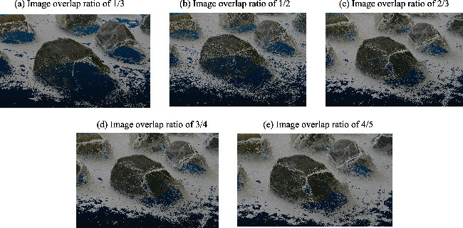
Fig. 1 Comparison between different three-dimensional (3D) reconstruction results with image overlap ratios of 1/3 (a), 1/2 (b), 2/3 (c), 3/4 (d), and 4/5 (e) |
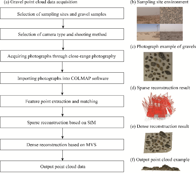
Fig. 2 Flowchart of gravel point cloud data acquisition (a) and pictures showing the sampling site environment (b), collected gravels (c), sparse reconstruction result based on Structure-from-Motion (SfM) (d), dense reconstruction result based on Multi-View Stereo (MVS) (e), and output point cloud data (f) |
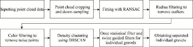
Fig. 3 Flowchart of gravel point cloud segmentation. RANSAC, Random Sample Consensus; DBSCAN, Density-Based Spatial Clustering of Applications with Noise. |
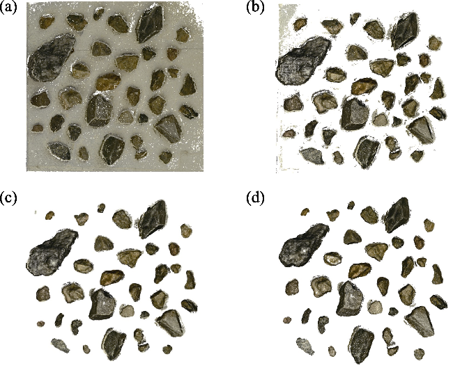
Fig. 4 Process of eliminating ground points from original gravel point clouds (a) using the RANSAC algorithm (b), radius filtering (c) and color filtering (d) |
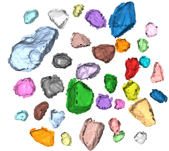
Fig. 5 Segmented gravel point cloud obtained using the DBSCAN algorithm. Each color represents a distinct gravel particle. |
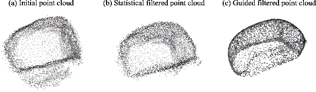
Fig. 6 Filtering schematic for a specific gravel particle (gravel number 15). (a), initial point cloud with noise points after segmentation; (b), statistical filtered point cloud; (c), guided filtered point cloud. |
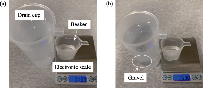
Fig. 7 Measurement of gravel volume using drainage method. (a), mass of the spilled water without the gravel; (b), mass of the spilled water with the gravel. |
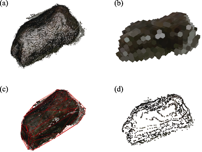
Fig. 8 Schematic diagram of gravel volume measurements based on the gravel point cloud (a) using the voxel raster method (b), convex packet method (c), and slicing method (d) |
Table 2 Description of 3D shape parameters of the gravel |
| Parameter | Equation | Description |
|---|---|---|
| Flatness | $F=\frac{A+B}{\text{2}C}$ | F is the flatness, with smaller F values indicating a flatter gravel shape; and A (mm), B (mm), and C (mm) are the grain sizes on X-axis, Y-axis and Z-axis, respectively. |
| Roundness | $I=\frac{{{A}_{p}}}{4\text{ }\!\!\pi\!\!\text{ }{{\left( \frac{A+B+C}{6} \right)}^{2}}}$ | I is the roundness; Ap (mm2) represents the actual surface area of the gravel and was calculated using point cloud triangulation, and the denominator means the surface area of the sphere with a diameter equal to the average of A, B, and C. |
| Sphericity | $\text{ }\!\!\rho\!\!\text{ }=\frac{{{d}_{n}}}{{{d}_{s}}}$ | ρ is the sphericity; dn (mm) represents the diameter of the sphere with the same volume as the gravel; ds (mm) is the diameter of the external sphere. The closer the sphericity is to 1, the closer the gravel resembles a perfect sphere. |
| Equivalent grain size | ${{D}_{F}}=\sqrt[3]{6V\text{/ }\!\!\pi\!\!\text{ }}$ | DF (mm) is the gravel's equivalent grain size, which is the diameter of a sphere with the same volume as the gravel, serving as a representative measure of the grain size; and V (mm3) represents the volume of the gravel. |
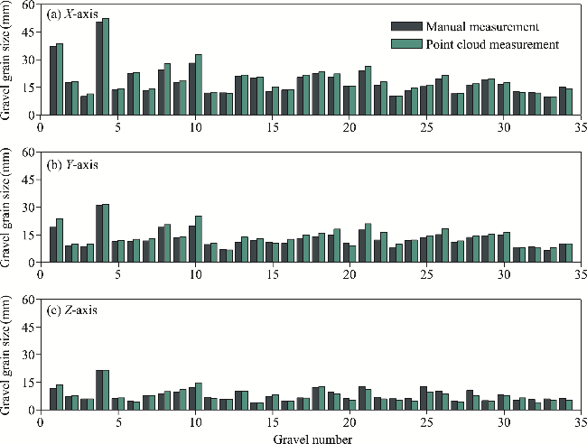
Fig. 9 Comparison between point cloud and manual measurements of the gravel grain sizes on X-axis (a), Y-axis (b), and Z-axis (c) |
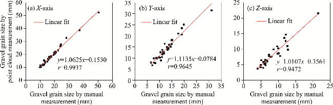
Fig. 10 Linear fit results of the gravel grain sizes between point cloud and manual measurements on X-axis (a), Y-axis (b), and Z-axis (c). r, Pearson's correlation coefficient. |
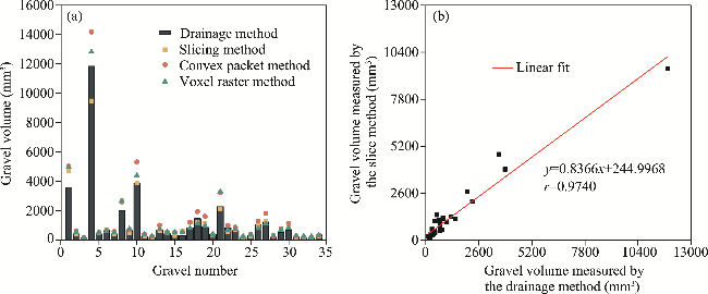
Fig. 11 Gravel volume measured by the drainage method, point cloud slicing method, convex packet method, and voxel raster method (a) and linear fit result of the volume measured by the drainage method and the slice method (b) |
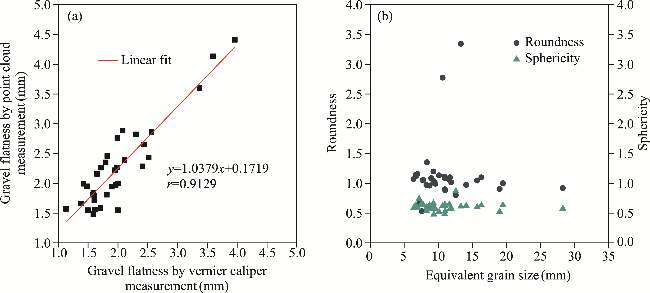
Fig. 12 Linear fit of gravel flatness measured by point cloud and vernier caliper (a) and distribution of gravel roundness and sphericity versus equivalent grain size of different gravel particles measured by point cloud (b) |
| [1] |
|
| [2] |
|
| [3] |
|
| [4] |
|
| [5] |
|
| [6] |
|
| [7] |
|
| [8] |
|
| [9] |
|
| [10] |
|
| [11] |
|
| [12] |
|
| [13] |
|
| [14] |
|
| [15] |
|
| [16] |
|
| [17] |
|
| [18] |
|
| [19] |
|
| [20] |
|
| [21] |
|
| [22] |
|
| [23] |
|
| [24] |
|
| [25] |
|
| [26] |
|
| [27] |
|
| [28] |
|
| [29] |
|
| [30] |
|
| [31] |
|
| [32] |
|
| [33] |
|
| [34] |
|
| [35] |
|
| [36] |
|
| [37] |
|
| [38] |
|
| [39] |
|
| [40] |
|
| [41] |
|
| [42] |
|
| [43] |
|
| [44] |
|
| [45] |
|
| [46] |
|
| [47] |
|
| [48] |
|
| [49] |
|
| [50] |
|
| [51] |
|
| [52] |
|
| [53] |
|
| [54] |
|
| [55] |
|
| [56] |
|
| [57] |
|
/
| 〈 |
|
〉 |