Full Length Article

Spatial differentiation and risk zonation of debris flow hazards in Tajikistan

  • JIA Wenjun a ,
  • CHEN Ningsheng , a, * ,
  • XUE Yang a ,
  • WANG Zhihan a ,
  • WEN Tao a ,
  • GUO Ru b ,
  • Safaralizoda NOSIR c ,
  • Aminjon GULAKHMADOV d
Expand
  • aInternational Cooperation Center for Mountain Multi-Disasters Prevention and Engineering Safety, School of Geosciences, Yangtze University, Wuhan, 430100, China
  • bSchool of Geosciences, Yangtze University, Wuhan, 430100, China
  • cInstitute of Geology, Earthquake-Resistant Construction and Seismology, National Academy of Sciences of Tajikistan, Dushanbe, 734000, Tajikistan
  • dInstitute of Water Problems, Hydropower and Ecology of the National Academy of Sciences of Tajikistan, Dushanbe, 734000, Tajikistan
* E-mail address: (CHEN Ningsheng).

Received date: 2025-10-09

  Revised date: 2025-12-22

  Accepted date: 2026-01-05

  Online published: 2026-03-11

Abstract

Debris flow events are frequent in Tajikistan, yet comprehensive investigations at the regional scale are limited. This study integrates remote sensing, Geographic Information System, and machine learning techniques to evaluate debris flow susceptibility and associated hazards across Tajikistan. A dataset comprising 405 documented debris flow points and 14 influencing factors, encompassing geological, climatic-hydrological, and anthropogenic variables, was established. Three machine learning algorithms—Random Forest, Support Vector Machine (SVM), and Multi-layer Perceptron—were applied to generate susceptibility maps and delineate debris flow risk zones. The results indicate that the areas of higher and high susceptibility accounted for 20.43% and 4.41% of the national area, respectively, and were predominantly concentrated along the Zeravshan and Vakhsh river basins. Among the evaluated models, SVM model demonstrated the highest predictive performance. Beyond conventional topographic and environmental controls, drought conditions were identified as a critical factor influencing debris flow occurrence within the arid and semi-arid mountainous regions of Tajikistan. These findings provide a scientific basis for regional debris flow risk management and disaster mitigation planning, and offer practical guidance for selecting conditioning factors in machine-learning-based susceptibility assessments in other dry mountainous environments.

Cite this article

JIA Wenjun , CHEN Ningsheng , XUE Yang , WANG Zhihan , WEN Tao , GUO Ru , Safaralizoda NOSIR , Aminjon GULAKHMADOV . Spatial differentiation and risk zonation of debris flow hazards in Tajikistan[J]. Regional Sustainability, 2026 , 7(1) : 100299 . DOI: 10.1016/j.regsus.2026.100299

1. Introduction

Debris flows are episodic, high-magnitude geohazards that predominantly occur in mountainous catchments. Their inherent unpredictability and destructive force pose formidable threats to human safety, socio-economic assets, and the operational integrity of critical infrastructure (Baggio et al., 2024). Central Asia, specifically Tajikistan, represents a prototypical high-risk zone characterized by complex orogeny, distinct hydro-climatic regimes, and intensifying anthropogenic interventions, which collectively catalyze frequent debris flow occurrences (Erokhin et al., 2018; Leinss et al., 2021). Recently, the perturbation of climate patterns has exacerbated extreme precipitation events, leading to an escalation in both the frequency and severity of debris flows. This trajectory presents systemic challenges to regional socio-economic development and ecological security (Sorg et al., 2012). For example, on 12 May 2021, continuous heavy rainfall triggered debris flows in Khatlon Province, Tajikistan, causing at least eight deaths and damaging multiple houses, farmlands, bridges, and highways (Xinhua News Agency, 2021). On 27 August 2023, intense rainfall induced debris flows killed 11 people in Vahdat City and 2 people in Rudaki District, Tajikistan, buried 15 vehicles, and forced the evacuation of hundreds of residents (Safarov et al., 2025).
However, the systematic characterization of the spatial distribution and deterministic drivers of debris flows in Tajikistan is nascent, largely constrained by monitoring lacunae and a dearth of comprehensive baseline datasets. This evidentiary gap impedes the efficacy of early warning systems and regional risk governance. To bolster disaster mitigation and resilience, there is an urgent need to develop high-fidelity susceptibility assessment models and execute rigorous scientific risk zonation.
In recent decades, debris flow susceptibility has attracted increasing scholarly attention due to its systemic threat to human safety, infrastructure, and the sustainable development of mountainous regions (Yılmaz et al., 2023; Shahgedanova et al., 2024). Traditional methods for debris flow susceptibility assessment can be broadly categorized into the following groups. First, methods based on empirical knowledge and historical disaster records. Researchers delineate susceptible areas according to the frequency, magnitude, and spatial distribution of debris flows, often combined with field surveys and remote sensing interpretation (Carrara et al., 2008; Kappes et al., 2011; Horton et al., 2013). However, these approaches rely heavily on long-term observational data and are therefore difficult to apply in data-scarce regions, such as high-mountain valleys, given the complex and variable nature of debris-flow environments. Second, multi-criteria evaluation methods based on topographic, geological, and hydrological factors, including analytic hierarchy process (Chen et al., 2015), fuzzy logic models (Zhang et al., 2022), and composite index approaches (Rogelis and Werner, 2014). These methods can integrate information from multiple sources but are strongly dependent on expert judgment, introducing subjectivity. Third, methods based on statistical and probabilistic theory, such as frequency ratio (Angillieri, 2020), information value (Xu et al., 2013), weight-of-evidence (Ilia and Tsangaratos, 2016), and logistic regression models (Bregoli et al., 2015). These approaches are more objective and operationally feasible, but they often assume independence among variables, making it challenging to capture nonlinear relationships and handle high-dimensional data effectively. Fourth, numerical simulation methods based on mathematical-physical processes, including finite element (Naef et al., 2006), finite difference (Shen et al., 2018), discrete element (Li et al., 2012), and coupled hydrodynamic models (Wei et al., 2024). Such methods can realistically represent the physical processes of debris flows, but their complexity, high parameter requirements, and computational demands usually limit their application to small-scale or typical catchments for hazard assessment and zoning.
With advances in geospatial data and computing technology, quantitative approaches integrating Geographic Information System (GIS), remote sensing, and statistical models have been widely applied to delineate debris flow-prone areas. However, traditional approaches exhibit several limitations. Empirical equations and regression-based models often fail to capture nonlinear interactions among conditioning factors, making them unsuitable for regions with strong spatial heterogeneity (Meng et al., 2024; Wang et al., 2025). Likewise, physically based numerical simulations, although theoretically rigorous, are highly sensitive to parameter uncertainty, boundary conditions, and computational requirements, which restricts their applicability for large-scale susceptibility assessment (Ma et al., 2022). In contrast, machine learning models can effectively handle high-dimensional, multi-source, and nonlinear datasets, providing improved predictive performance compared with traditional empirical and statistical methods (Meng and Zhu, 2024; Xie et al., 2025b). More recently, algorithms such as Random Forest (RF) (Huang et al., 2022b), Support Vector Machine (SVM) (Zhao et al., 2024), and Multi-layer Perceptron (MLP) (Yang et al., 2024) have been increasingly adopted for susceptibility mapping. Despite their advantages, challenges remain in transferring machine learning models across different regions, incorporating environmental change scenarios, and improving interpretability of the underlying physical mechanisms.
Selecting appropriate conditioning factors is essential for model accuracy. A widely accepted assumption is that higher precipitation correlates with increased debris flow frequency. However, recent observations in arid and semi-arid regions suggest that severe events may also occur under drought-dominated conditions (Zhou et al., 2024). Study in the Tianshan Mountains has shown that large-scale debris flows can be triggered even with limited precipitation input (Hu et al., 2017), a phenomenon reported in other dry mountainous regions globally (Handwerger et al., 2019). This implies that prolonged drought may influence slope stability by altering soil properties and promoting the accumulation of loose deposits. Despite this, drought conditions have rarely been incorporated into susceptibility assessments, particularly in Central Asia. Considering the arid climate of Tajikistan, integrating a drought index into susceptibility modeling is both necessary and scientifically justified.
Building upon these research gaps, this study incorporates a drought index along with 13 other environmental factors to develop a comprehensive debris flow susceptibility assessment for Tajikistan. Using remote sensing, GIS, and multiple machine learning models, we perform susceptibility modeling, spatial differentiation analysis, and disaster risk zoning. The findings aim to provide a scientific basis and technical support for debris flow prevention, control, and emergency management in mountainous countries of Central Asia.

2. Study area

Tajikistan is located in the southeastern part of Central Asia (36°40′-41°05′N, 67°31′-75°14′E). It borders China to the east, Kyrgyzstan to the north, Uzbekistan to the west, and Afghanistan to the south, with a total land area of approximately 143,100 km2. The terrain generally decreases in elevation from east to west (Fig. 1), encompassing three major mountain systems: the Pamir Plateau, the western margin of the Hindu Kush Mountains, and the southern Tianshan Mountains. It is one of the most rugged countries in the world, with mountains accounting for more than 93.00% of the total area. Major river valleys, such as the Vakhsh and Panj rivers, develop along fault zones. Their erosive action has deeply incised the mountains, forming characteristic gorges and alluvial fans. During periods of intense rainfall or snowmelt, these geomorphic and hydrological settings make the region highly susceptible to debris flow hazards.
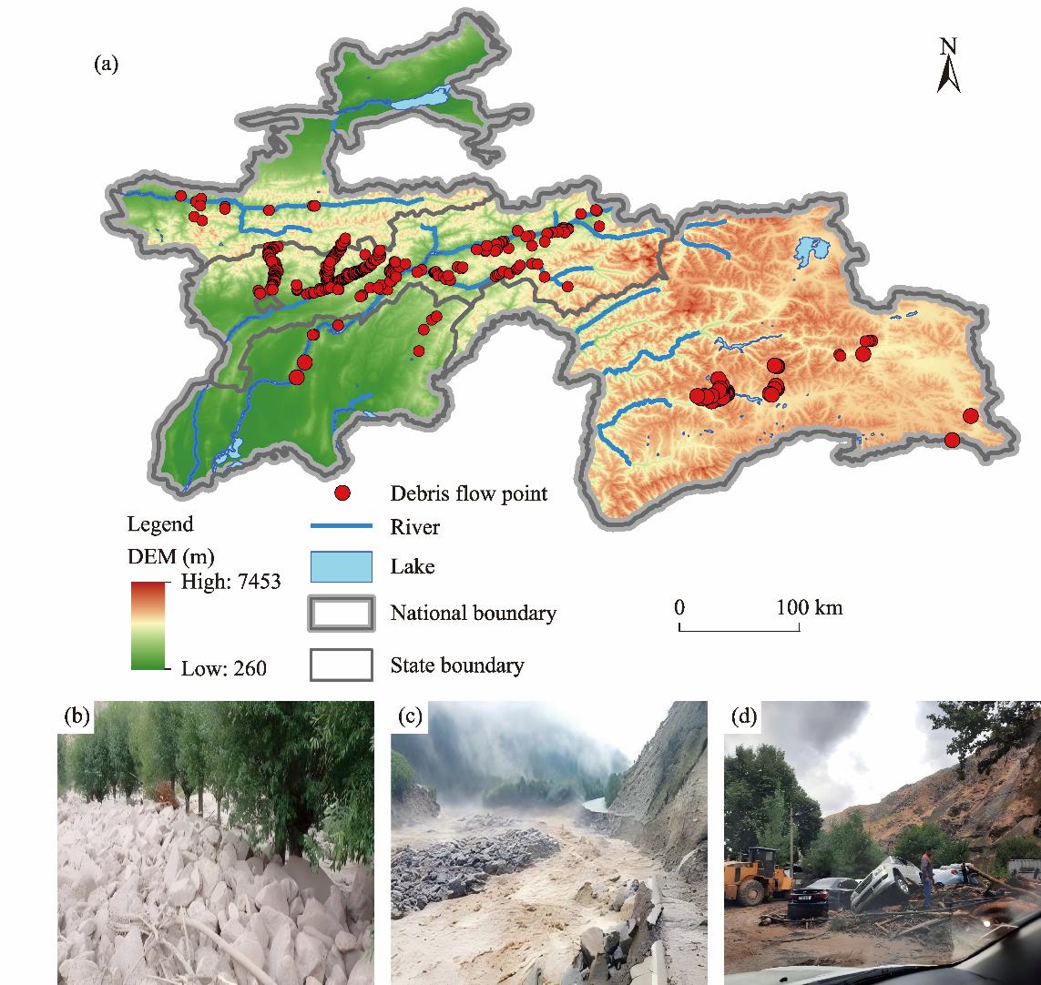
Fig. 1. Overview of debris flow disasters in Tajikistan. (a), study area and distribution of debris flow points; (b), gravel deposited around tree trunks following a debris flow; (c), road destroyed by the debris flow; (d), trees and vehicles destroyed by the debris flow. DEM, digital elevation model. Note that the national boundary and state boundary were obtained from the Global Administrative Areas (GADM) database version 4.2 (http://www.gadm.org/), which provides generalized boundaries and does not explicitly represent disputed or undetermined borders. The boundary of the standard map used in this study has not been modified.
Debris flow disasters in Tajikistan are mainly concentrated in areas where steep mountainous terrain and deeply incised river valleys converge (Fig. 1). Typical examples include the Zeravshan River and its upper reaches in the Gissar Mountains (such as Panjakent City, Ayni District, and Ghafurov District), as well as the Rasht Valley zone (including Rasht District and Nurobod District). These regions are generally characterized by high elevation, strong relief, and a dense gully network. These river valleys are characterized by steep slopes that provide abundant loose material. When subjected to heavy rainfall or snowmelt, the resulting surface runoff readily converges and mobilizes sediment, leading to debris flow disasters.
Compelling evidence from a recent study indicates that climate change has directly amplified the threat of debris flows in Central Asia’s mountainous regions, particularly within Tajikistan (Shahgedanova et al., 2024). Rising air temperatures and accelerated cryosphere degradation have altered hydrological regimes, increased meltwater contributions, and enlarged the supply of loose debris on steep slopes, thereby enhancing the likelihood of channelized debris-flow formation (Lin et al., 2025; Shen et al., 2025). Concurrently, climate-driven perturbations in precipitation patterns—specifically the increased periodicity of high-intensity, short-duration rainfall—serve as pivotal triggers for debris flows in high-relief catchments. These evolving hydro-geomorphic dynamics substantially exacerbate the susceptibility of the fragile Pamir Plateau and Gissar Mountain valleys, where inherent geological instability and an abundance of lithogenic debris predispose the terrain to mass wasting. Such climate-related impacts underscore the urgency of conducting updated susceptibility assessments to better understand debris flow dynamics under ongoing environmental change.
The stratigraphy of Tajikistan is predominantly composed of sedimentary rocks and displays pronounced lithological diversity (Fig. 2). Quaternary units are mainly represented by unconsolidated deposits composed of mud, clay, sand, gravel, alluvium, and silt. These materials are widely distributed across intermontane basins, plains, and major river valleys, where they are closely associated with modern fluvial systems and surface geomorphological processes. Paleozoic strata are extensively exposed in the eastern and southwestern mountainous regions. These formations are dominated by carbonate rocks, particularly limestone and dolomite, and are commonly interbedded with slate, siltstone, and sandstone. In some areas, Paleozoic sequences also include volcanic and intrusive rocks such as diabase, dacite, and tuff, reflecting complex tectono-magmatic activity. Mesozoic formations are primarily concentrated in western Tajikistan and some intermontane basins. Their lithological assemblages mainly consist of sandstone, siltstone, conglomerate, and limestone, with localized occurrence of evaporitic minerals such as gypsum, consistent with sedimentation under variable depositional environments. Cenozoic deposits, including Paleogene and Neogene units, are widely distributed in tectonically active foreland and basin regions. These strata are characterized by thick clastic successions composed predominantly of conglomerate, sandstone, siltstone, and clay, reflecting intensive uplift, erosion, and sediment accumulation processes. In addition, extensive Quaternary glacial deposits occur in high-altitude regions, where glaciers currently occupy approximately 6.70% of the national territory. Meltwater from these glaciers constitutes an important hydrological source during the warm season and plays a critical role in the generation of floods and debris flows.
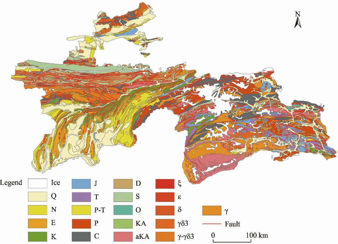
Fig. 2. Geological map of Tajikistan. Stratigraphic units are categorized as follows: Q (Quaternary): unconsolidated deposits mainly composed of mud, clay, sand, gravel, alluvium, and silt; N (Neogene): sandstone, conglomerate, and clay; E (Paleogene): variegated clays, sandstone, siltstone, dolomite, gypsum, conglomerate, and limestone; K (Cretaceous): redstone, siltstone, clay, conglomerates, and limestone; J (Jurassic): limestone, sandstone, silt, gypsum, and siltstone; T (Triassic): variegated sandstones, conglomerate, and siltstone; P-T (Permian-Triassic): limestone, sandstone, siltstone, and conglomerate; P (Permian): limestone, sandstone, tuff, slate, diabase, and marl; C (Carboniferous): limestone, slate, siltstone, sandstone, dacite, diabase, tuff, and andesite; D (Devonian): dolomite, limestone, slate, and chert; S (Silurian): slate, limestone, dolomite, diabase, and porphyrite; O (Ordovician): slate, sandstone, and siltstone; KA (Cambrian): slate, limestone, siltstone, and sandstone; aKA (Precambrian): quartzite, feldspathic quartzite, and sericite; ξ: monzogranite; ε: ultrabasic complex; δ: diorite; γδ3: granodiorite; γ-γδ3: granodiorite-granite; γ, granodiorite.

3. Data and methodology

The methodological framework, encompassing data processing, computational procedures, and modeling techniques, is illustrated in Figure 3. The research workflow is organized into five primary stages: (1) compiling a comprehensive debris flow inventory based on existing datasets, supplemented by satellite imagery interpretation and field surveys; (2) conducting multicollinearity diagnostics to select characteristic variables relevant to debris flow initiation; (3) constructing predictive susceptibility models using machine learning algorithms; (4) evaluating and validating model performance through comparative analysis; and (5) integrating risk assessments for exposed elements, specifically road density and population density.
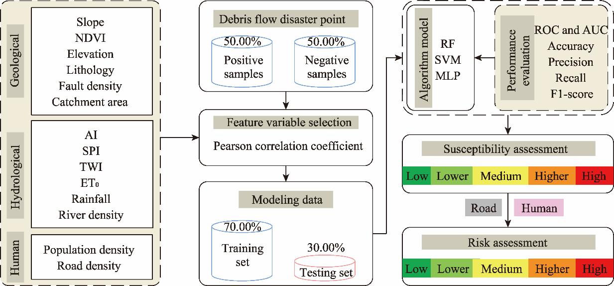
Fig. 3. Flow chart of this study. NDVI, Normalized Difference Vegetation Index; AI, Aridity Index; SPI, Stream Power Index; TWI, Topographic Wetness Index; ET0, potential evapotranspiration; RF, Random Forest; SVM, Support Vector Machine; MLP, Multi-layer Perceptron; ROC, Receiver Operating Characteristic; AUC, Area under the ROC curve; F1-score, harmonic mean of precision and recall.

3.1. Data sources

The national boundaries used in all maps were obtained from the Global Administrative Areas (GADM) database version 4.2 (http://www.gadm.org/), which provides high-quality, widely accepted administrative boundary data for countries worldwide. This dataset ensures the accuracy of spatial analysis and mapping in this study. All maps were generated using these boundaries to maintain consistency and reproducibility.
A total of 405 debris flow points were used for machine learning modeling in the debris flow susceptibility assessment. These points were primarily obtained from historical records, visual interpretation, and field investigations. The morphology of alluvial fans and catchments can be used to preliminarily distinguish debris flows from fluvial fans. We conducted preliminary selection through the interpretation of Google Earth imagery, based on the following minimum thresholds used to differentiate debris flows from flood channels: a Melton ratio greater than 0.6 for catchments and a slope greater than 3.3° for fans (Wilford et al., 2004). In some catchments, satellite imagery was obscured by shadows, making it difficult to accurately identify debris flow points. To verify the accuracy of remote sensing interpretation, field investigations were conducted during May-June in 2025.
While hazards like landslides are often idealized as point features, debris flows are inherently catchment-scale processes. Therefore, this study adopts catchments as the evaluation units to better capture the completeness of influencing factors (Fig. 4). Catchments where debris flows occurred were assigned a label value of 1, while those without debris flow occurrences were assigned a label value of 0. The dataset was split into training (70.00%) and testing (30.00%) sets following common practice. Both sets were balanced, maintaining a 1:1 ratio between debris-flow catchments (positive samples) and non-debris-flow catchments (negative samples).
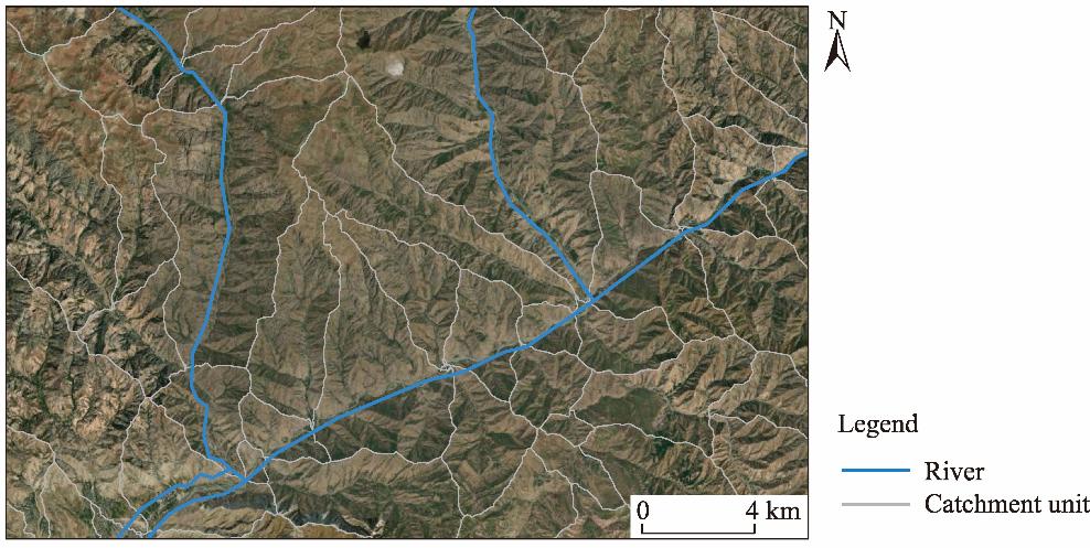
Fig. 4. Catchment units with an area larger than 1 km2 extracted via Geographic Information System (GIS) platform.

3.2. Selection of influencing factors

The occurrence of debris flows is influenced by multiple factors, including hydrology, geomorphology, and geology. In this study, a total of 14 characteristic variables were selected, including catchment area, elevation, slope, vegetation index (i.e., Normalized Difference Vegetation Index (NDVI)), lithology, fault density, precipitation, river density, Aridity Index (AI), potential evapotranspiration (ET0), Stream Power Index (SPI), Topographic Wetness Index (TWI), population density, and road density (Fig. 5). Based on the dominant lithologies of different geological periods, we classified the lithology of Tajikistan into six categories according to rock strength: granite, diorite, slate, siltstone, ice/snow, and clay. Except for catchment area, the detailed physical meaning and data sources of the remaining characteristic variables are summarized in Table 1.
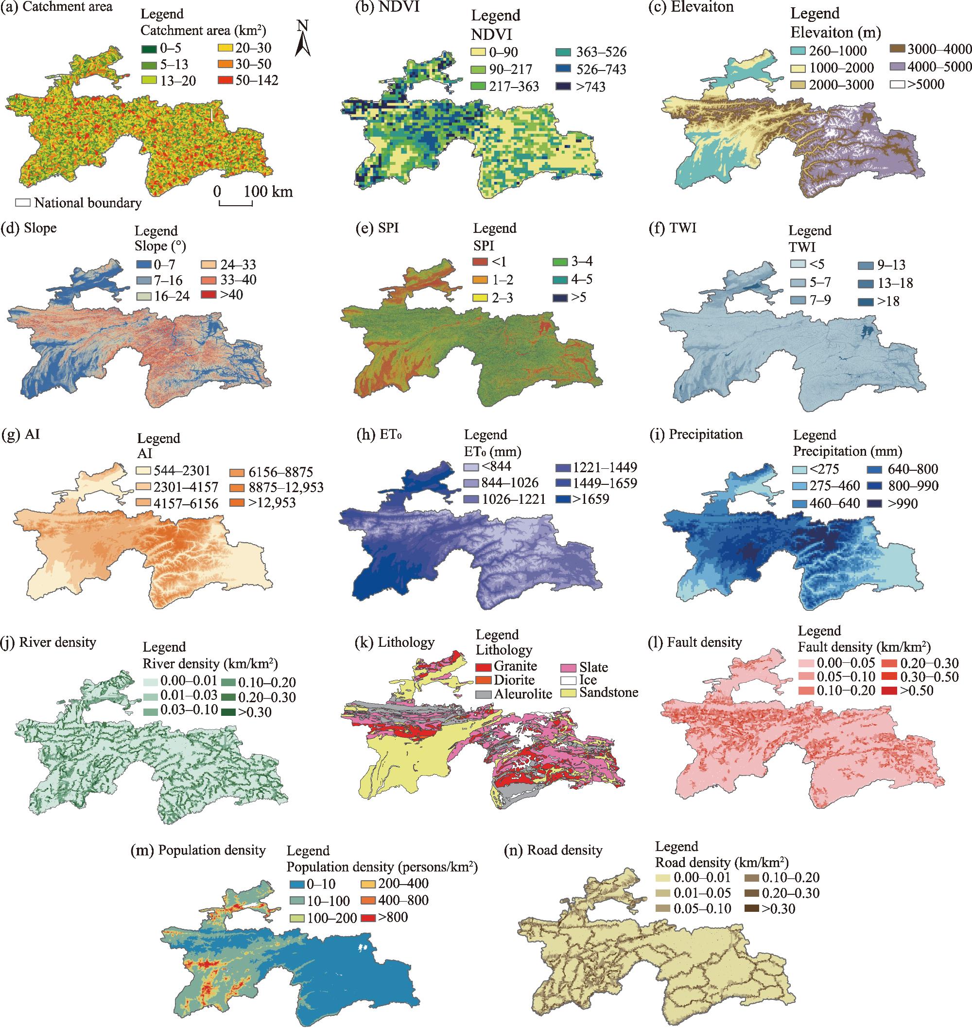
Fig. 5. Spatial distribution of debris flow influencing factors. (a), catchment area; (b), NDVI; (c), elevation; (d), slope; (e), SPI; (f), TWI; (g), AI; (h), ET0; (i), precipitation; (j), river density; (k), lithology; (l), fault density; (m), population density; (n), road density. Note that the national boundary and state boundary were obtained from the GADM database version 4.2 (http://www.gadm.org/), which provides generalized boundaries and does not explicitly represent disputed or undetermined borders. The boundary of the standard map used in this study has not been modified.
Table 1 Characteristic variables selected in this study.
Factor type Factor name Effect on debris flow activity Data source
Geological factor Elevation (m) Mountainous terrain supplies abundant loose material and features steep slopes, thereby elevating the probability of debris flow occurrence. Elevation was extracted from the 30 m resolution digital elevation model (DEM) provided by United States Geological Survey (USGS) (https://earthexplorer.usgs.gov/)
Slope (°) Steeper slopes enhance gravity-driven mass movement, leading to slope instability and rapid downslope sliding. Calculated from DEM in ArcGIS software (version 10.8; Esri, Inc., Redlands, the USA)
Normalized Difference Vegetation Index (NDVI) The NDVI reflects vegetation coverage. Li et al. (2023)
Lithology Loose deposits or weak rocks are easily eroded by rainfall, providing abundant source materials for debris flows. 1:150,000 geological map (Academy of Sciences of the Tajik SSR,1968)
Fault density (km/km2) Faults influence the degree of bedrock fragmentation. For linear variables, fault density indicates the total fault length per unit area (Huang et al., 2022a). Calculated from 1:150,000 geological map of Tajikistan (Academy of Sciences of the Tajik SSR, 1968)
Climatic and hydrological factor Precipitation (mm) Precipitation denotes the total cumulative precipitation in 2024. WorldClim (https://www.worldclim.org/data/worldclim21.html)
River density (km/km2) Dense river networks facilitate runoff concentration and may erode gully toes, triggering debris flows. National Earth System Science Data Center (https://www.geodata.cn/main/)
Aridity Index
(AI)
The AI is an indicator of climatic dryness, defined as the ratio of water loss to water supply. Arid conditions can cause surface cracking, enhance rainfall infiltration into slopes, and promote debris flow initiation. Figshare (https://doi.org/10.6084/m9.figshare.7504448.v5)
Potential evapotranspiration (ET0; mm) The ET0 affects soil moisture and vegetation growth; areas with lower ET0 are more likely to retain higher water content. Figshare (https://doi.org/10.6084/m9.figshare.7504448.v5)
Stream Power Index (SPI) The SPI reflects the erosive power of flowing water, calculated as:
$\text{SPI}=\mathrm{ln}\left(\alpha \times \mathrm{tan}\beta \right)$
,
where α is the upslope contributing area (m2); and β is the slope (°).
Calculated from DEM in ArcGIS software
Topographic Wetness Index
(TWI)
The TWI characterizes soil moisture conditions in a catchment, calculated as:
$\text{TWI}=\mathrm{ln}\left(\alpha /\mathrm{tan}\beta \right)$
.
Calculated from DEM in ArcGIS software
Human activities Population density (persons/km2) Concentrated human activities may disturb slope stability and increase debris flow risk. WorldPop Hub
(https://hub.worldpop.org/geodata/)
Road density (km/km2) Road construction and excavation may weaken slope structure, alter drainage pathways, and enhance debris flow hazards. National Earth System Science Data Center (https://www.geodata.cn/main/)
Catchment area (km2) Catchment area serves as the evaluation unit for debris flows. Calculated from DEM in ArcGIS software
To facilitate machine learning modeling, a comprehensive dataset was constructed by integrating environmental covariates with their corresponding slope stability states. Missing values in the environmental factor layers were subjected to spatial interpolation; where reliable estimation was not feasible, a constant value of -32,767 was assigned. The finalized dataset was partitioned into a training set (70.00%) and a testing set (30.00%). Finally, all variables were standardized to a range of 0.0-1.0 through min-max normalization to ensure computational convergence during model training.

3.3. Machine learning algorithms

3.3.1. Random Forest (RF)

RF is an ensemble learning architecture based on a multitude of decision trees. By aggregating the outputs of individual trees through voting (classification) or averaging (regression), RF enhances predictive accuracy and effectively mitigates the risk of overfitting. Its primary advantages include high resilience to outliers, the capability to process high-dimensional datasets without prior feature selection, and the inherent capacity to quantify the relative importance of conditioning factors.

3.3.2. Supporting Vector Machine (SVM)

SVM is a supervised learning algorithm grounded in the structural risk minimization principle and the maximum- margin hyperplane concept (Xie et al., 2025a). SVM delineates optimal boundaries between disparate categories by identifying a hyperplane that maximizes the inter-class margin in the feature space. To address non-linear complexities, kernel functions can be employed to map original data into higher-dimensional feature spaces. In this study, the Gaussian kernel function was selected because it effectively captures non-linear relationships with fewer hyper-parameter requirements compared to polynomial kernel functions, thereby reducing computational overhead and numerical instability. Consequently, the Gaussian kernel function was utilized throughout SVM modeling and prediction phases.

3.3.3. Multi-layer Perceptron (MLP)

MLP is a typical feedforward artificial neural network consisting of an input layer, one or more hidden layers, and an output layer (Meng et al., 2023). By using nonlinear activation functions and the backpropagation algorithm, the model can approximate complex nonlinear relationships, making it suitable for both classification and regression tasks. The hidden layer of MLP processes information via a neurons network interconnected by weighted links. A sigmoid nonlinear activation function is incorporated to facilitate the learning of intricate patterns. Through iterative training cycles employing optimization techniques, such as the backpropagation algorithm and gradient descent, the model refines its weights and biases to minimize the discrepancy between predicted outputs and actual targets. The number of hidden layers and the maximum number of iterations are determined via hyper-parameter tuning.

3.4. Hyper-parameter optimization

In this study, the Tree-structured Parzen Estimator (TPE) algorithm, implemented via the Optuna framework, was employed to systematically optimize the key hyper-parameters for each model. To ensure statistical robustness, each tuning trial was executed in triplicate, with the optimal configuration selected for final model deployment. The pre-defined search space for these hyper-parameters is detailed in Table 2.
Table 2 Statistics of hyper-parameter adjustment range.
Model Hyper-parameter Range Step
Random Forest (RF) n_estimators 30.00000-800.00000 1.00000
max_depth 10.00000-60.00000 1.00000
max_features 10.00000-60.00000 1.00000
min_impurity_decrease 0.00000-5.00000 0.10000
Supporting Vector Machine (SVM) kenel ‘rbf’ -
degree 500.00000-2000.00000 1.00000
gamma 0.00100-0.30000 0.00001
coef0 10.00000-30.00000 0.10000
tol 0.05000-0.30000 0.00100
C 10.00000-40.00000 0.01000
Multi-layer Perceptron (MLP) hidden_layer_sizes 10.00000-200.00000 1.00000
max_iter 500.00000-2000.00000 10.0000
alpha 0.00010-0.70000 0.00010
learning_rate 0.00010-0.65000 0.00010

Note: -, no data.

The optimization process was conducted in two sequential phases. Initially, a coarse-tuning exploration was performed by partitioning the theoretical parameter ranges into discrete intervals to identify high-performance zones. Subsequently, a fine-grained search was executed within these refined intervals (Table 2). Initial broad-spectrum experiments indicated that the optimal parameters consistently converged within the specified search space, validating that our selected ranges adequately encapsulate the data characteristics of the study area. While further expansion of the search space or reduction of the step size might yield infinitesimal gains, the associated escalation in computational cost would yield diminishing returns. This balanced approach aligns with the efficiency principles of the TPE algorithm, ensuring high predictive performance without incurring unnecessary computational latency.

3.5. Model performance evaluation

A confusion matrix is a tool that presents the prediction results of a classification model in matrix form, where rows represent the actual classes and columns represent the predicted classes. By counting the number of true positives (TP), true negatives (TN), false positives (FP), and false negatives (FN), the prediction performance of the model for each class can be intuitively reflected. TP and TN represent the number of correctly classified debris flow and non-debris flow samples, respectively, while FP and FN represent the number of misclassified debris flow and non-debris flow samples, respectively. The Receiver Operating Characteristic (ROC) curve has been widely used to validate susceptibility prediction models. The ROC curve plots the true positive rate (TPR) on the Y-axis against the false positive rate (FPR) on the X-axis. The Area under the ROC curve (AUC) provides a quantitative benchmark for model accuracy, with values ranging from 0.5 to 1.0. The higher the AUC, the better the model performance; when AUC approaches 1.0, the model achieves higher precision.
In addition to the above metrics, accuracy, precision, recall, and the harmonic mean of precision and recall (F1-score) were also considered as performance indicators of the models.
Accuracy is defined as the ratio of correctly predicted samples to the total number of samples, reflecting the overall correctness of the predictions. The formula is:
$\text{Accuracy=}\frac{\text{TP+TN}}{\text{TP+TN+FP+FN}}$
where TP is the number of positive samples correctly predicted as positive; TN is the number of negative samples correctly predicted as negative; FP is the number of negative samples incorrectly predicted as positive; and FN is the number of positive samples incorrectly predicted as negative.
Precision (%) is the proportion of correctly predicted positive samples among all samples predicted as positive, reflecting the reliability of the prediction results. The formula is:
$\text{Precision=}\frac{\text{TP}}{\text{TP+FP}}$
Recall (%) is the proportion of correctly predicted positive samples to the total number of actual positive samples, which measures the model’s ability to detect positive instances. The formula is:
$\text{Recall=}\frac{\text{TP}}{\text{TP+FN}}$
F1-score is the harmonic mean of precision and recall, providing a comprehensive measure of both the accuracy and completeness of the model. The formula is:
$\text{F1-score=}2\times \frac{\text{Precision}\times \text{Recall}}{\text{Precision+Recall}}$
To rigorously evaluate the significance of these performance differentials, this study employed DeLong’s test and Bootstrap permutation test. DeLong’s test, a robust non-parametric method, yields a test statistic and corresponding P-value to determine if the divergence between estimators surpasses the threshold of random fluctuation. This approach effectively accounts for inter-model correlations, making it particularly suitable for comparing machine learning classifiers trained on the same dataset, especially when AUC variations are subtle (Demler et al., 2012). A P-value less than 0.05 in DeLong’s test signifies statistical significance at the 0.05 level, allowing rejection of the null hypothesis and concluding that the observed differences are not due to random errors.
Complementarily, the Bootstrap permutation test offers a more generalized resampling-based approach to estimate the distribution of model statistics. By generating 1000 resampled datasets with replacement, this method facilitates an empirical assessment of performance without assuming a specific population distribution (Janssen and Pauls, 2003). If the resulting 95.00% confidence interval (CI) for the performance difference is entirely positive, the former model is deemed significantly superior. Conversely, a CI entirely below zero indicates the statistical superiority of the latter model, whereas a CI that includes zero suggests no significant difference between the two models at the specified confidence level.
All models presented in this study were trained and evaluated on a workstation featuring an Intel(R) Core (TM) i5-13500 central processing unit (CPU), an NVIDIA GeForce 1650 graphics processing unit (GPU), and running Windows 10. The development environment was based on Python software (version 3.8.1; Python Software Foundation, Wilmington, the USA). Specifically, MLP algorithm was implemented using PyTorch (version 1.10.0; Meta AI, Inc., Menlo Park, the USA), RF and SVM algorithms were implemented using scikit-learn (version 1.3.2; INRIA, Rocquencourt, France), while the TPE algorithm was implemented using Optuna software (version 4.4.0; Preferred Networks, Inc., Tokyo, Japan).

4. Results

4.1. Characteristic variables collinearity

Figure 6 shows the Pearson correlation coefficients among the 14 characteristic variables. The correlation coefficient between ET0 and elevation was -0.871, indicating a strong negative correlation. After excluding ET0, the remaining 13 variables were used for model training and validation.
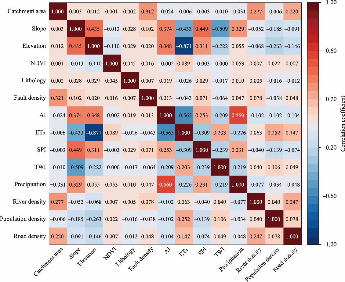
Fig. 6. Pearson correlation between characteristic variables.

4.2. Spatial distribution characteristics of debris flow hazards in Tajikistan

The relationship between debris-flow distribution and regional characteristics was analyzed by quantifying, for each variable, the number of occurrences and their corresponding areal proportion (Fig. 7). This quantification provides a basis for further examination.
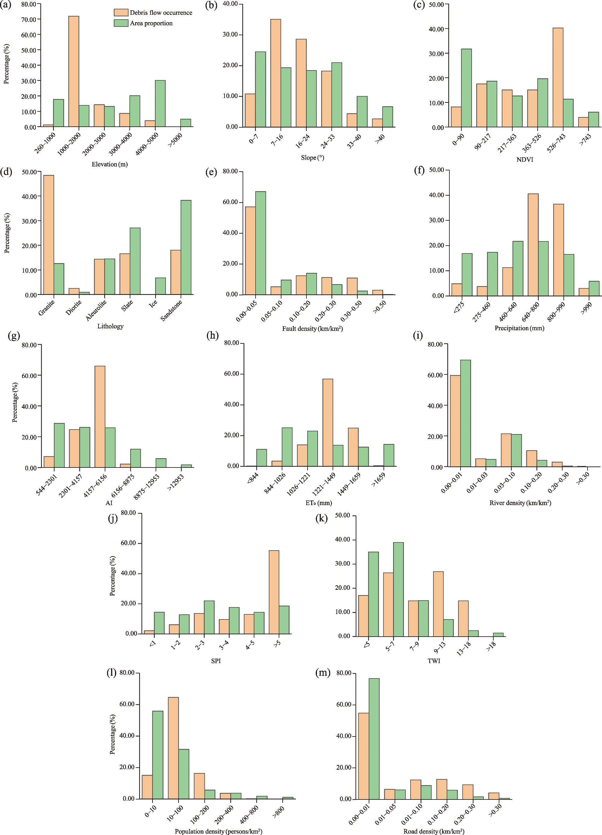
Fig. 7. Distribution of debris flow occurrence and area proportion across different environmental factors. (a), elevation; (b), slope; (c), NDVI; (d), lithology; (e), fault density; (f), precipitation; (g), AI; (h), ET0; (i), river density; (j), SPI; (k), TWI; (l), population density; (m), road density.
Debris flow formation in Tajikistan was strongly controlled by geological and geomorphological conditions, including elevation, slope, vegetation cover, lithology, and fault density. Debris flow occurrences were predominantly concentrated within the elevation range of 1000-2000 m, accounting for 71.85% of the total inventory. Moderate slopes (7°-24°) represented the most active susceptibility window, hosting 63.70% of the recorded events. Approximately 40.25% of debris flows were distributed in areas with NDVI values between 526 and 743. Notably, lithology exerted a profound influence, with granite regions exhibiting the highest density of occurrences; while these regions occupied only 12.60% of the total area, they contained 48.40% of all debris flows. In terms of structural geology, 57.14% of debris flows occurred in zones with a fault density of 0.00-0.05 km/km2. This high percentage was partly because areas with very low fault density constitute a large portion of the country. However, the incidence rate showed an overall upward trajectory as fault density increased, indicating that tectonic activity significantly governs the initiation of debris flows.
Climatic and hydrological factors play a critical role in debris flow development by regulating water availability, runoff generation, and erosive capacity across catchments. Regions with precipitation of 640-800 and 800-990 mm accounted for 40.60% and 36.47% of debris flows events, respectively. Both figures significantly exceeded their respective areal proportions, identifying these medium-to-high rainfall zones as highly prone to debris flow activity. Debris flows were primarily situated in areas with sparse river density (<0.01 km/km2), representing 59.40% of events. Catchments with an AI between 4157 and 6156 contained 65.93% of debris flows events, suggesting that moderate moisture levels and episodic concentrated rainfall favor both material accumulation and rapid runoff generation. Similarly, areas with ET0 values of 1221-1449 mm hosted 56.79% of debris flows events despite covering only 13.78% of the territory. Elevated SPI values, which signify enhanced fluvial erosive power, combined with higher regional humidity, facilitated runoff concentration and sediment entrainment. Furthermore, while areas with TWI values of 9-13 covered only 7.08% of the study area, they accounted for 26.91% of debris flows events, underscoring the critical role of water convergence capacity in hazard risk.
Human activities exerted an additional influence on debris flow occurrence by modifying slope stability, surface conditions, and hydrological responses in mountainous regions. Regions with a population density of 10-100 persons/km2 occupy 31.58% of the area but disproportionately contained 64.60% of debris flow locations. This suggests that within this demographic threshold, anthropogenic interventions strongly intersect with natural geomorphic processes, contributing to increased disaster frequency. Conversely, areas with low road density (0.00-0.01 km/km2) accounted for 76.76% of the territory and 54.89% of debris flows events, indicating that a substantial portion of events still occurs within relatively undisturbed or pristine natural landscapes.

4.3. Susceptibility assessment results

The susceptibility maps generated by the three algorithms were classified into five levels—low, lower, medium, higher, and high—using the natural breaks method. Figure 8 illustrates the spatial distribution of debris flow susceptibility across the study area for each algorithm. The proportion of area in each susceptibility category varied among the three algorithms: MLP model exhibited the largest proportion of high-susceptibility areas (6.94%), followed by SVM (4.41%) and RF (3.72%). Despite differences in area proportions across individual levels, the combined proportion of higher and high susceptibility zones was broadly consistent among the three models, with SVM, MLP, and RF accounting for 24.83%, 17.78%, and 21.27%, respectively. Spatially, the higher and high susceptibility zones identified by all three algorithms showed a broadly similar pattern, predominantly aligned along the northwest Zeravshan River and central Vakhsh River. These areas are characterized by moderate slopes and elevation differences, coupled with relatively low precipitation and high aridity, making them particularly prone to debris flow occurrence.
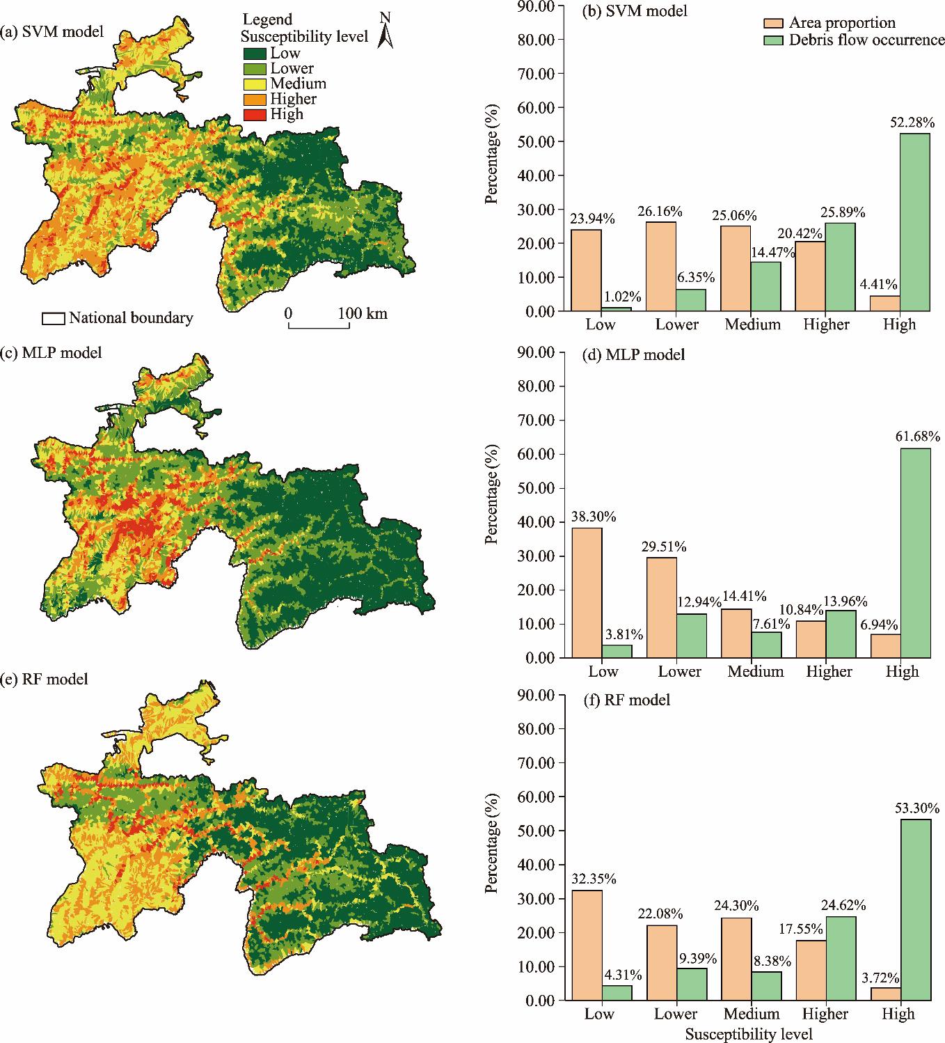
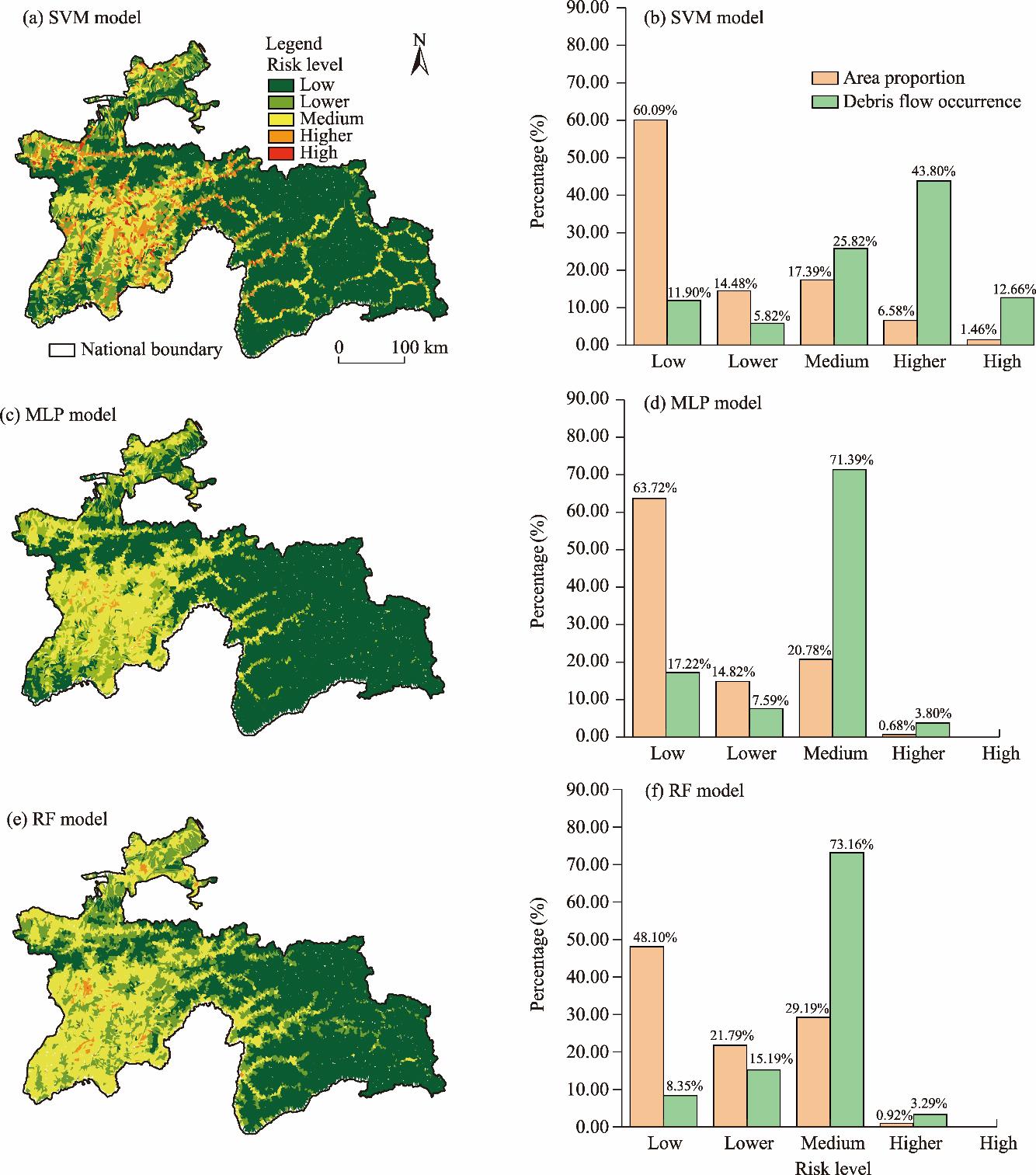
Fig. 8. Debris flow susceptibility assessment based on three machine learning algorithms. (a, c, and e), spatial distribution of debris flow susceptibility based on SVM model, MLP model, and RF model, respectively; (b, d, and f), comparison between area proportion and debris flow occurrence across different susceptibility levels based on SVM model, MLP model, and RF model, respectively. Note that the national boundary and state boundary were obtained from the GADM database version 4.2 (http://www.gadm.org/), which provides generalized boundaries and does not explicitly represent disputed or undetermined borders. The boundary of the standard map used in this study has not been modified.

4.4. Model verification and performance comparison

Figure 9 presents the confusion matrices for the training and testing sets constructed using the three algorithms. In these matrices, the green-shaded areas indicate predictions that match the actual data. It can be observed that all three models performed well on both the training and testing sets, with predictive accuracy for the testing sets exceeding 79.17%, indicating satisfactory predictive performance. These results confirm the reliability of the susceptibility maps generated earlier (Fig. 8) and support the robustness of the models in capturing the key controlling factors of debris flow hazards across the study area.
Fig. 9. Confusion matrices of the three machine-learning models. (a and b), training set and testing set in SVM model, respectively; (c and d), training set and testing set in RF model, respectively; (e and f), training set and testing set in MLP model, respectively. TP (true positive), the number of debris flow samples correctly predicted as debris flows; TN (true negative), the number of non-debris flow samples correctly predicted as non-debris flows; FP (false positive), the number of non-debris flow samples incorrectly predicted as debris flows; FN (false negative), the number of debris flow samples incorrectly predicted as non-debris flows. The percentages in each column were normalized by the total number of actual samples per class (column-wise proportions). These values indicate the model’s sensitivity (true positive rate) in the first column and specificity (true negative rate) in the second column.
The validation metrics mentioned above are summarized in Table 3. The performance differences among the three models on the training and testing sets were minor, indicating that their generalization capabilities were relatively stable. Overall, SVM model achieved the best performance in terms of accuracy and F1-score, reflecting its balanced capability in optimizing both precision and recall. MLP model exhibited high accuracy on both training and testing sets, with good precision, but relatively lower recall, indicating that some positive samples may be missed. RF model achieved the highest precision, suggesting reliable prediction of positive samples; however, its lower recall resulted in a reduced F1-score. Overall, SVM model provided a balanced performance across all metrics, making it more suitable for debris flow susceptibility prediction.
Table 3 Static validation of confusion matrix on three models.
Model Set Accuracy Precision Recall F1-score
MLP Training set 0.73102 0.74038 0.36150 0.48579
Testing set 0.74342 0.79167 0.35849 0.49351
SVM Training set 0.76733 0.86000 0.40376 0.51952
Testing set 0.75000 0.82609 0.35849 0.50000
RF Training set 0.71122 0.75676 0.26291 0.39024
Testing set 0.73026 0.83333 0.28320 0.42253

Note: F1-score, harmonic mean of precision and recall.

Figure 10 presents the ROC curves for the training and testing sets for all the three algorithms. Among them, SVM model achieved the highest AUC of 0.77, whereas MLP and RF models both achieved an AUC of 0.75. This indicates that SVM model slightly outperforms the other two models on the testing set. MLP model showed the highest AUC on the training set, reflecting stronger fitting ability to the training set but a slight decline on the testing set, suggesting a potential risk of overfitting. Overall, all three models demonstrated stable classification performance, with SVM model achieving the best testing accuracy while maintaining minimal AUC differences between training and testing sets, highlighting its robust generalization capability for debris flow susceptibility mapping.
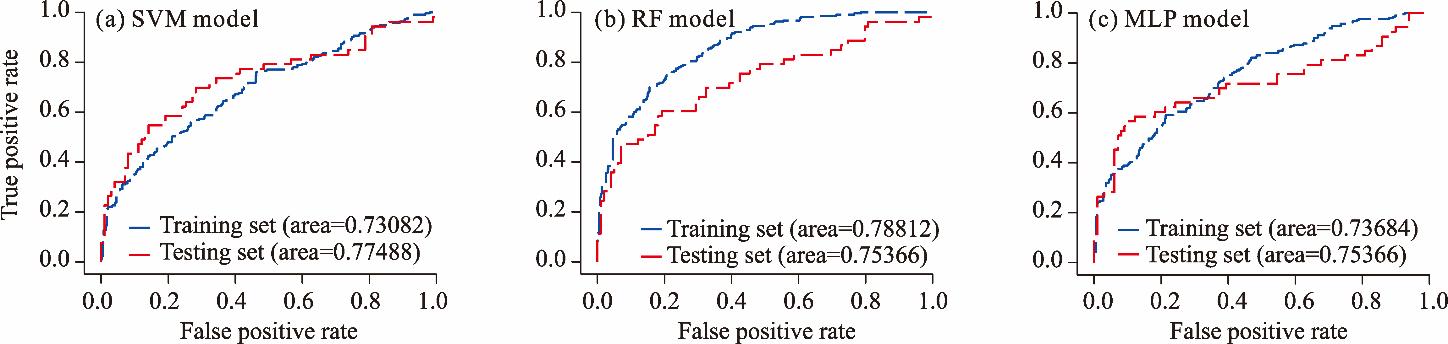
Fig. 10. Receiver Operating Characteristic (ROC) curve of three models. (a), SVM model; (b), RF model; (c), MLP model.
While Table 3 and Figure 10 reveal numerical variances in accuracy and AUC values among SVM, MLP, and RF models, these marginal discrepancies do not inherently imply statistical significance. Consequently, it remains ambiguous whether the observed variations originate from stochastic noise or reflect the divergent predictive capabilities of the models.
The results detailed in Table 4 elucidate that SVM model exhibited statistically significant performance advantages over both MLP and RF models, as corroborated by both DeLong’s test and Bootstrap permutation test. In all pairwise comparisons, SVM model demonstrated a clear and statistically robust superiority, suggesting that its predictive outputs are the most reliable for debris flow susceptibility mapping. Furthermore, the significance tests between MLP and RF models indicated that RF model significantly outperformed MLP model. Collectively, these findings validated that the observed accuracy and AUC gaps between SVM and its counterparts were statistically significant. The superior performance of SVM model was thus credible, attributable to the model’s inherent architectural advantages rather than stochastic variability.
Table 4 Comparison of model performance using DeLong’s test and Bootstrap permutation test.
Model comparison Set P-value (from DeLong’s test) 95.00% CI (from Bootstrap permutation test)
SVM vs. MLP Training set <0.001 (0.43019, 0.46114)
SVM vs. MLP Testing set <0.001 (0.13491, 0.21950)
SVM vs. RF Training set 0.030 (1.08170×10⁻⁶, 1.54030×10⁻⁵)
SVM vs. RF Testing set <0.001 (0.07010, 0.13108)
MLP vs. RF Training set <0.001 (-0.46115, -0.43019)
MLP vs. RF Testing set <0.001 (-0.31723, -0.23814)

Note: CI, confidence interval.

4.5. Risk assessment and zoning

Following the natural breaks method, exposed elements were categorized into five risk levels, and combined with debris flow susceptibility classes, a risk matrix was constructed to classify debris flow risk into five levels (Table 5).
Table 5 Risk assessment matrix integrating debris flow susceptibility and exposed element categories.
Exposed element
1 2 3 4 5
Susceptibility 1 Low Low Lower Medium Medium
2 Low Lower Medium Medium Higher
3 Lower Medium Medium Higher Higher
4 Medium Medium Higher Higher High
5 Medium Higher Higher High High
Figure 11 presents the spatial distribution of risk zonation based on population density. In terms of areal extent, the low- and lower-risk zones constituted the dominant proportions across all three algorithms. Specifically, the low-risk zone encompassed 48.10% in RF model, 60.09% in SVM model, and 63.72% in MLP model. These findings suggested that the majority of the territory was characterized by either sparse population or low debris flow susceptibility, resulting in a relatively low overall regional risk profile. Medium-risk zones occupied 29.19% of the area in RF model, while appearing comparatively smaller in SVM and MLP models. In contrast, the spatial footprints of higher- and high-risk zones were marginal, yet SVM results demonstrated higher sensitivity in demarcating these critical areas, identifying 6.58% and 1.46% as higher and high risk, respectively.
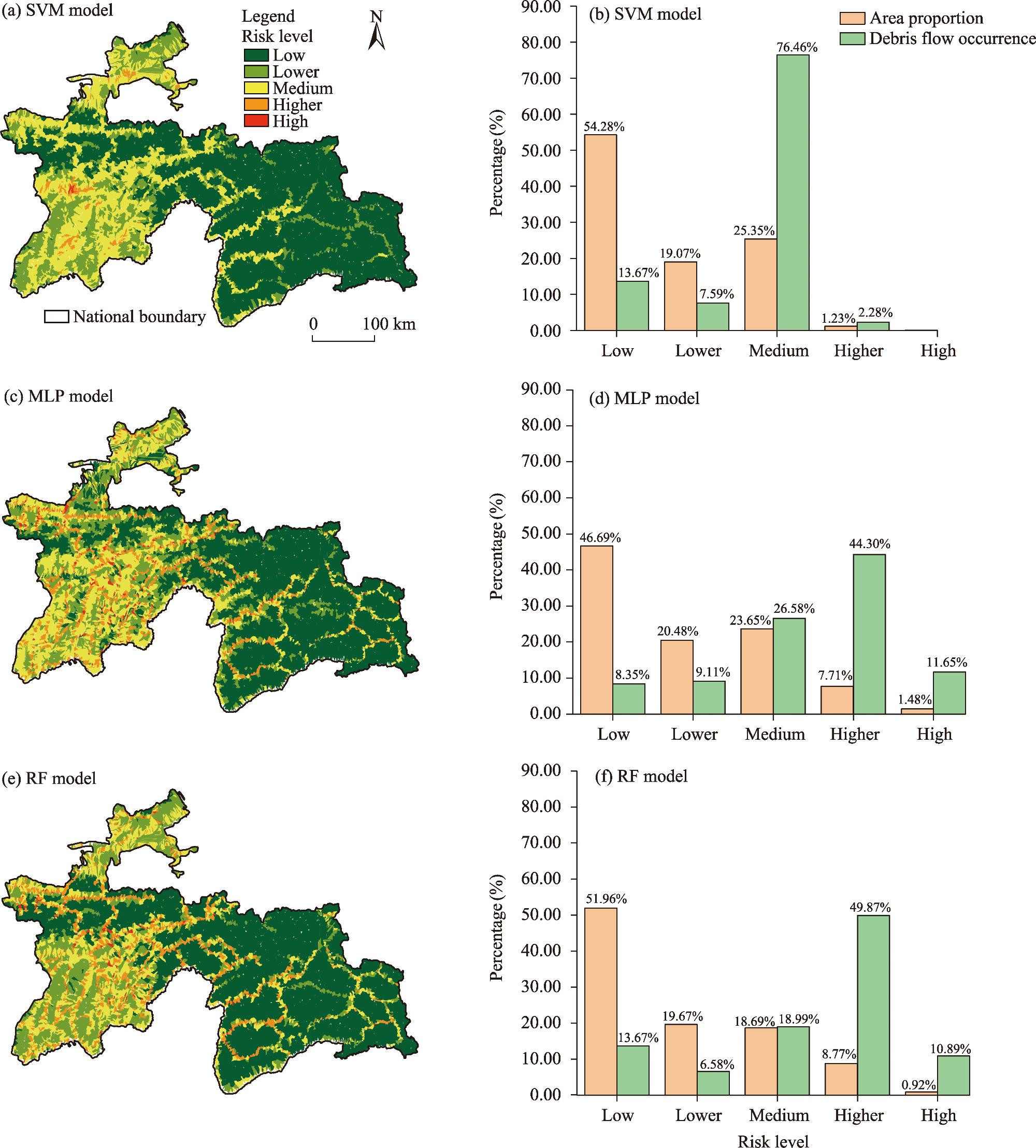
Fig. 11. Debris flow hazard risk based on population density. (a, c, and e), risk zoning based on population density in SVM model, MLP model, and RF model, respectively; (b, d, and f), area proportion of different hazard levels and the corresponding distribution of historical debris flows in SVM model, MLP model, and RF model, respectively. Note that the national boundary and state boundary were obtained from the GADM database version 4.2 (http://www.gadm.org/), which provides generalized boundaries and does not explicitly represent disputed or undetermined borders. The boundary of the standard map used in this study has not been modified.
To further validate the geographical accuracy of these models, the distribution of historical debris flow occurrences was integrated into the risk framework. The results indicated that the distribution of historical disasters was generally congruent with the classified risk levels. In RF and MLP models, the medium-risk zones exhibited the highest concentration of historical events, reaching 73.16% and 71.39%, respectively. This confirmed that these zones captured a substantial portion of actual disaster hotspots, reflecting a robust recognition of moderate-risk areas. Conversely, in SVM model, higher- and high-risk zones hosted 43.80% and 12.66% of historical debris flows, respectively—values that significantly exceeded their respective areal proportions. This disproportionate representation highlights the superior capacity of SVM model for high-risk identification.
Across all three algorithms, the spatial patterns of risk were consistent: low and lower-risk areas were primarily located in the uninhabited, high-altitude regions of the eastern Pamir Plateau and the central Gissar-Alay Mountains. Medium-risk areas were aligned with fluvial corridors in the east and high-relief canyon zones or tectonically active regions in the west. Notably, higher- and high-risk zones were concentrated in the vicinity of Dushanbe City and along the densely populated Zeravshan and Vakhsh river basins, underscoring the intersection of geomorphic hazards and anthropogenic vulnerability.
Figure 12 illustrates the risk zonation results derived from road density analysis. Regarding the distribution of road segments across risk categories, the low-risk class constituted the predominant share: 51.96% in RF model, 54.28% in SVM model, and 46.69% in MLP model. This indicated that the majority of the regional transportation network traversed areas with relatively high geomorphic stability. While the proportion of higher- and high-risk segments remained modest, notable inter-model variations emerged: RF and MLP models identified 9.67% and 9.19% of segments as higher or high risk, respectively, whereas SVM model provided a more conservative estimate of 1.29%.
Fig. 12. Debris flow hazard risk based on road density. (a, c, and e), risk zoning based on road density in SVM model, MLP model, and RF model, respectively; (b, d, and f), area proportion of different hazard levels and the corresponding distribution of historical debris flows in SVM model, MLP model, and RF model, respectively. Note that the national boundary and state boundary were obtained from the GADM database version 4.2 (http://www.gadm.org/), which provides generalized boundaries and does not explicitly represent disputed or undetermined borders. The boundary of the standard map used in this study has not been modified.
A comparative analysis of the spatial outputs reveals that in SVM model, high-risk zones were principally clustered around Dushanbe City. Although the relatively subdued topography in this vicinity reduced the inherent susceptibility to gully-type debris flows, the dense concentration of population and infrastructure synergistically elevated the aggregate risk. Conversely, RF and MLP models indicated that medium-to-higher risk zones largely overlapped with corridors of high road density. Given that extensive road segments were engineered along fluvial valleys—often situated at the confluence of drainage lines and active gullies—they possessed an inherent capacity for pluvial convergence. Such topographic positioning renders transportation infrastructure highly vulnerable to runoff accumulation during extreme precipitation, thereby triggering debris flow events.

5. Discussion

By normalizing the contribution weights across the machine learning algorithms, the relative importance of environmental covariates was elucidated (Fig. 13). Elevation was consistently identified as the predominant deterministic factor across all three algorithms, underscoring that topographic relief provides the requisite gravitational potential energy for debris flow initiation. In contrast, variables such as catchment area, NDVI, and precipitation exhibited relatively lower importance. The secondary drivers were identified as the AI, fault density, slope, and lithology. Fault density is intrinsically linked to geological friability and rock mass fragmentation, as tectonic activity generates fractured substrates, thereby ensuring a profuse sediment supply. While slope primarily governs mass transport kinematics, lithology dictates the weathering intensity, both of which are directly coupled with the sediment budgets required for debris flow mobilization.
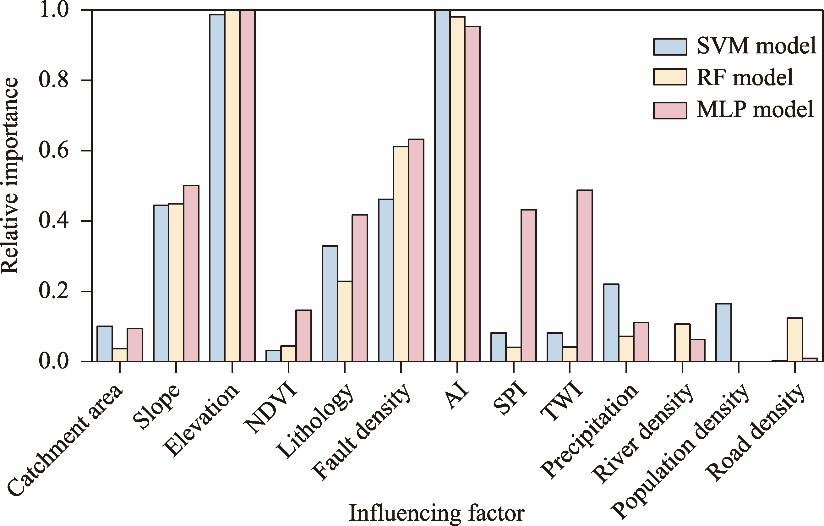
Fig. 13. Relative importance of the characteristic variables.
While extant literature frequently identifies rainfall intensity as the primary trigger for debris flows (Zhao et al., 2021), the influence of antecedent drought remains critically under-researched. However, post-drought debris flows are increasingly recognized as a global phenomenon. Similar to observations in southwestern China and Colombia (Nyman et al., 2019; Chen et al., 2020a), Tajikistan is a hotspot for drought-conditioned mass movements. This region’s semi-arid climate, characterized by desiccated summers followed by intense autumnal convective storms (Podgórski et al., 2023), facilitates high runoff coefficients and severe soil erosion.
Our findings suggest that drought exerts a more profound structural control on debris flow occurrence than instantaneous precipitation. We posit that while precipitation provides the immediate hydrological impulse, initiation is fundamentally governed by sediment availability (Liu et al., 2020). Prolonged water deficits induce desiccation cracking, enhance mechanical weathering, and attenuate soil cohesion, thereby compromising the structural integrity of hillslopes. These drought-induced fissures act as preferential flow paths, allowing rapid infiltration during subsequent storms, which triggers abrupt spikes in pore-water pressure (Hu et al., 2019; Zhong et al., 2021). Concurrently, drought-mediated vegetation degradation weakens root reinforcement and promotes the accumulation of loose proluvial materials. When extreme, short-duration precipitation follows a protracted dry spell—a characteristic climatic pulse in Tajikistan—the convergence of weakened slope stability, abundant lithogenic debris, and rapid runoff concentration creates an optimal environment for debris flow initiation. The transition from drought-induced soil weakening to rainfall-triggered mobilization (Chen et al., 2020b) represents a critical sediment-supply shift that is often overlooked in traditional susceptibility frameworks.
The catchment-scale susceptibility maps identify the Zeravshan and Vakhsh river basins as national-level hazard hotspots, providing a scientific basis for government agencies to prioritize targeted monitoring and engineering mitigation. Furthermore, the demonstrated impact of hydro-climatic coupling highlights the necessity of incorporating soil-moisture deficits and drought indices into early-warning systems, rather than relying exclusively on rainfall thresholds. Integrating real-time aridity monitoring with high-resolution meteorological forecasts would enable authorities to identify “windows of heightened vulnerability” more accurately (Chen et al., 2022; Li et al., 2024).
Several caveats warrant consideration. First, the AI used here represents a long-term climatological baseline rather than a dynamic, temporally resolved measure of antecedent moisture states. Consequently, it reflects the background aridity regime rather than event-specific hydrological fluctuations. Future research should integrate multi-temporal metrics (e.g., SPI time series or satellite-derived soil moisture anomalies) to better quantify how drought-rainfall transitions modulate hazards (Ren and Leslie, 2020). Second, while machine learning models effectively capture spatial risks, challenges regarding sample imbalance and hyper-parameter sensitivity persist (Dikshit et al., 2021). Finally, data resolution remains a decisive constraint (Zhang et al., 2019). Although 30 m resolution was utilized, it may bypass fine-scale geomorphic nuances. As higher-resolution datasets for both topography and precipitation become more accessible, the predictive fidelity and operational reliability of machine learning-based assessments are expected to improve significantly.

6. Conclusions

This study executed a systematic regional-scale assessment of debris flow hazards in Tajikistan, utilizing hydrological catchments as the fundamental mapping units. By integrating three machine learning algorithms— SVM, RF, and MLP—we evaluated debris flow susceptibility and further synthesized these outputs with population and transportation data to construct a multi-dimensional risk zonation framework. This research aims to elucidate the deterministic drivers of debris flows and provide a robust scientific foundation for disaster risk reduction in data-scarce mountainous environments.
The empirical findings demonstrate that while geological and geomorphological configurations provide foundational controls on debris flow initiation, hydro-climatic factors modulate their spatio-temporal variability. Furthermore, human activities, specifically road density and population density, exert a significant footprint on regional hazard profiles. Among the evaluated models, SVM model exhibited superior predictive fidelity and spatial discrimination, successfully capturing 56.46% of historical events within a mere 8.04% of the total land area. High-risk hotspots were predominantly clustered in the Zeravshan and Vakhsh river basins—regions characterized by the convergence of steep topography, lithological complexity, and intense anthropogenic pressure. Notably, beyond traditional topographic variables, antecedent drought conditions emerged as a pivotal factor, underscoring their critical role in preconditioning slope failure through material weakening.
Based on these outcomes, we recommend that priority should be accorded to high-risk catchments in the formulation of monitoring protocols, early warning systems, and structural mitigation strategies. Future research should prioritize the integration of dynamic hydro-climatic indicators and multi-temporal remote sensing observations to enhance model robustness. Such advancements will be essential for supporting adaptive disaster risk management and fostering socio-ecological resilience amidst accelerating environmental transformations in Central Asia.

Authorship contribution statement

JIA Wenjun: data curation, formal analysis, methodology, resources, software, validation, visualization, and writing - original draft; CHEN Ningsheng: supervision, project administration, and funding acquisition; XUE Yang: investigation, resources, supervision, and writing - review & editing; WANG Zhihan: data curation, software, methodology, and validation; WEN Tao: project administration, resources, and supervision; GUO Ru: validation; Safaralizoda NOSIR: investigation and resources; and Aminjon GULAKHMADOV: investigation and resources. All authors approved the manuscript.

Declaration of conflict of interest

The authors declare that they have no known competing financial interests or personal relationships that could have appeared to influence the work reported in this paper.

Acknowledgements

This study was supported by the National Natural Science Foundation of China (42361144880), the Science and Technology Program of Xizang Autonomous Region, China (XZ202402ZD0001), and the Qinghai Province Basic Research Program Project, China (2024-ZJ-904). The authors would like to sincerely thank Dr. Ishfaq GUJREE for his professional assistance in improving the English language, clarity, and readability of the manuscript.
[1]
Academy of Sciences of the Tajik SSR (Soviet Socialist Republic), 1968. Atlas of the Tajik Soviet Socialist Republic. Dushanbe: Main Administration of Geodesy and Cartography (GUGK) (in Russian).

[2]
Angillieri M.Y.E., 2020. Debris flow susceptibility mapping using frequency ratio and seed cells, in a portion of a mountain international route, dry Central Andes of Argentina. CATENA. 189, 104504, doi: 10.1016/j.catena.2020.104504.

[3]
Baggio T., Martini M., Bettella F., et al., 2024. Debris flow and debris flood hazard assessment in mountain catchments. CATENA. 245, 108338, doi: 10.1016/j.catena.2024.108338.

[4]
Bregoli F., Medina V., Chevalier G., et al., 2015. Debris-flow susceptibility assessment at regional scale: Validation on an alpine environment. Landslides. 12, 437-454.

DOI

[5]
Carrara A., Crosta G., Frattini P., 2008. Comparing models of debris-flow susceptibility in the alpine environment. Geomorphology. 94(3-4), 353-378.

DOI

[6]
Chen H.Y., Ruan H.C., Chen J.G., et al., 2022. Review of investigations on hazard chains triggered by river-blocking debris flows and dam-break floods. Frontiers in Earth Science. 10, 83004, doi: 10.3389/feart.2022.830044.

[7]
Chen N.S., Zhang Y., Tian S.F., et al., 2020a. Effectiveness analysis of the prediction of regional debris flow susceptibility in post-earthquake and drought site. Journal of Mountain Science. 17(2), 329-339.

DOI

[8]
Chen X.Z., Chen H., You Y., et al., 2015. Susceptibility assessment of debris flows using the analytic hierarchy process method - A case study in Subao river valley, China. Journal of Rock Mechanics and Geotechnical Engineering. 7(4), 404-410.

DOI

[9]
Chen Y., Qin S.W., Qiao S.S., et al., 2020b. Spatial predictions of debris flow susceptibility mapping using convolutional neural networks in Jilin Province, China. Water. 12(8), 2079, doi: 10.3390/w12082079.

[10]
Demler O.V., Pencina M.J., D’Agostino Sr. R.B., et al., 2012. Misuse of DeLong test to compare AUCs for nested models. Statistics in Medicine. 31(23), 2577-2587.

[11]
Dikshit A., Pradhan B., Alamri A.M., 2021. Pathways and challenges of the application of artificial intelligence to geohazards modelling. Gondwana Research. 100, 290-301.

DOI

[12]
Erokhin S.A., Zaginaev V.V., Meleshko A.A., et al., 2018. Debris flows triggered from non-stationary glacier lake outbursts: the case of the Teztor Lake complex (Northern Tian Shan, Kyrgyzstan). Landslides. 15(1), 83-98.

DOI

[13]
Handwerger A.L., Huang M.H., Fielding E.J., et al., 2019. A shift from drought to extreme rainfall drives a stable landslide to catastrophic failure. Scientific Reports. 9(1), 1569, doi: 10.1038/s41598-018-38300-0.

PMID

[14]
Horton P., Jaboyedoff M., Rudaz B., et al., 2013. Flow-R, a model for susceptibility mapping of debris flows and other gravitational hazards at a regional scale. Natural Hazards and Earth System Sciences. 13(4), 869-885.

[15]
Hu G.S., Shang Y.J., Zeng Q.L., et al., 2017. The emergency scientific investigation of catastrophic debris flow in Yecheng County of Xinjiang on July 6th, 2016. Mountain Research. 35(1), 112-116.

[16]
Hu G.S., Zhao C.Y., Chen N.S., et al., 2019. Characteristics, mechanisms and prevention modes of debris flows in an arid seismically active region along the Sichuan-Tibet railway route, China: a case study of the Basu-Ranwu section, southeastern Tibet. Environmental Earth Sciences. 78(18), 564, doi: 10.1007/s12665-019-8554-z.

[17]
Huang F.M., Pan L.H., Fan X.M., et al., 2022a. The uncertainty of landslide susceptibility prediction modeling: suitability of linear conditioning factors. Bulletin of Engineering Geology and the Environment. 81, 182, doi: 10.1007/s10064-022-02672-5.

[18]
Huang H., Wang Y.S., Li Y.M., et al., 2022b. Debris-flow susceptibility assessment in China: A comparison between traditional statistical and machine learning methods. Remote Sensing. 14(18), 4475, doi: 10.3390/rs14184475.

[19]
Ilia I., Tsangaratos P., 2016. Applying weight of evidence method and sensitivity analysis to produce a landslide susceptibility map. Landslides. 13(2), 379-397.

DOI

[20]
Janssen A., Pauls T., 2003. How do bootstrap and permutation tests work? The Annals of Statistics. 31(3), 768-806.

[21]
Kappes M.S., Malet J.P., Remaître A., et al., 2011. Assessment of debris-flow susceptibility at medium-scale in the Barcelonnette Basin, France. Natural Hazards and Earth System Sciences. 11(2), 627-641.

[22]
Leinss S., Bernardini E., Jacquemart M., et al., 2021. Glacier detachments and rock-ice avalanches in the Petra Pervogo range, Tajikistan (1973-2019). Natural Hazards and Earth System Sciences. 21(5), 1409-1429.

[23]
Li C.J., Hu Y.X., Fan G., et al., 2024. Exploring debris flow deposit morphology in river valleys: Insights from physical modeling experiments. Engineering Geology. 332, 107465, doi: 10.1016/j.enggeo.2024.107465.

[24]
Li M.Y., Cao S., Zhu Z.C., et al., 2023. Spatiotemporally Consistent Global Dataset of the GIMMS Normalized Difference Vegetation Index (PKU GIMMS NDVI) from 1982 to 2022 (V1.2). [2025-08-30]. https://doi.org/10.5281/zenodo.8253971.

[25]
Li W.C., Li H.J., Dai F.C., et al., 2012. Discrete element modeling of a rainfall-induced flowslide. Engineering Geology. 149-150, 22-34.

DOI

[26]
Lin Y., Guo Z.H., Meng Q.B., et al., 2025. Prediction of peak strength under triaxial compression for sandstone based on ABC-SVM algorithm. Expert Systems with Applications. 264, 125923, doi: 10.1016/j.eswa.2024.125923.

[27]
Liu M., Zhang Y., Tian S.F., et al., 2020. Effects of loose deposits on debris flow processes in the Aizi Valley, southwest China. Journal of Mountain Science. 17(1), 156-172.

DOI

[28]
Ma T.X., Lin Y., Zhou X.B., et al., 2022. Grading evaluation of goaf stability based on entropy and normal cloud model. Advances in Civil Engineering. 2022(1), 9600909, doi: 10.1155/2022/9600909.

[29]
Meng D.B., Yang S.Y., De Jesus A.M.P., et al., 2023. A novel hybrid adaptive Kriging and water cycle algorithm for reliability-based design and optimization strategy: Application in offshore wind turbine monopile. Computer Methods in Applied Mechanics and Engineering. 412, 116083, doi: 10.1016/j.cma.2023.116083.

[30]
Meng D.B., Yang S.Y., Yang H.F., et al., 2024. Intelligent-inspired framework for fatigue reliability evaluation of offshore wind turbine support structures under hybrid uncertainty. Ocean Engineering. 307, 118213, doi: 10.1016/j.oceaneng.2024.118213.

[31]
Meng D.B., Zhu S.P., 2024. Multidisciplinary Design Optimization of Complex Structures Under Uncertainty. Boca Raton: CRC Press.

[32]
Naef D., Rickenmann D., Rutschmann P., et al., 2006. Comparison of flow resistance relations for debris flows using a one-dimensional finite element simulation model. Natural Hazards and Earth System Sciences. 6(1), 155-165.

[33]
Nyman P., Rutherfurd I.D., Lane P.N.J., et al., 2019. Debris flows in southeast Australia linked to drought, wildfire, and the El Niño-Southern Oscillation. Geology. 47(5), 491-494.

DOI

[34]
Podgórski J., Pętlicki M., Fernández A., et al., 2023. Evaluating the impact of the Central Chile mega drought on debris cover, broadband albedo, and surface drainage system of a dry Andes glacier. Science of The Total Environment. 905, 166907, doi: 10.1016/j.scitotenv.2023.166907.

[35]
Ren D.D., Leslie L.M., 2020. Climate warming enhancement of catastrophic southern California debris flows. Scientific Reports. 10(1), 10507, doi: 10.1038/s41598-020-67511-7.

PMID

[36]
Rogelis M.C., Werner M., 2014. Regional debris flow susceptibility analysis in mountainous peri-urban areas through morphometric and land cover indicators. Natural Hazards and Earth System Sciences. 14(11), 3043-3064.

[37]
Safarov M., Kang S.C., Fazylov A., et al., 2025. Mapping the territories of the mountain-foothill zone of Tajikistan exposed to mudflows. Journal of Mountain Science. 22(1), 16-30.

DOI

[38]
Shahgedanova M., Saidaliyeva Z., Mussina A., et al., 2024. Debris flows in the northern Tien Shan, Central Asia: regional database, meteorological triggers, and trends. npj Natural Hazards. 1, 49, doi: 10.1038/s44304-024-00050-7.

[39]
Shen L.X., Ma T.X., Chen H., et al., 2025. A new CNN-GRU deep learning framework optimized by CHIO for precise prediction of debris flow velocity. Stochastic Environmental Research and Risk Assessment. 39(6), 2351-2371.

DOI

[40]
Shen W., Li T.L., Li P., et al., 2018. A modified finite difference model for the modeling of flowslides. Landslides. 15(8), 1577-1593.

DOI

[41]
Sorg A., Bolch T., Stoffel M., et al., 2012. Climate change impacts on glaciers and runoff in Tien Shan (Central Asia). Nature Climate Change. 2, 725-731.

DOI

[42]
Wang Y.F., Ma T.X., Shen L.X., et al., 2025. Prediction of thermal conductivity of natural rock materials using LLE-transformer-lightGBM model for geothermal energy applications. Energy Reports. 13, 2516-2530.

DOI

[43]
Wei Z.L., Shang Y.Q., Liang Q.H., et al., 2024. A coupled hydrological and hydrodynamic modeling approach for estimating rainfall thresholds of debris-flow occurrence. Natural Hazards and Earth System Sciences. 24(10), 3357-3379.

[44]
Wilford D.J., Sakals M.E., Innes J.L., et al., 2004. Recognition of debris flow, debris flood and flood hazard through watershed morphometrics. Landslides. 1(1), 61-66.

[45]
Xie S.J., Lin H., Duan H.Y., et al., 2025a. A novel triaxial strength criterion for rocks based on the ultimate strength and its application. Geoenergy Science and Engineering. 246, 213590, doi: 10.1016/j.geoen.2024.213590.

[46]
Xie S.J., Lin H., Ma T.X., et al., 2025b. Prediction of joint roughness coefficient via hybrid machine learning model combined with principal components analysis. Journal of Rock Mechanics and Geotechnical Engineering. 17(4), 2291-2306.

DOI

[47]
Xinhua News Agency, 2021. Eight People Died in a Debris Flow in Tajikistan. [2025-07-15]. https://www.xinhuanet.com/world/2021-05/12/c_1127438295.htm?baike in Chinese).

[48]
Xu W.B., Yu W.J., Jing S.C., et al., 2013. Debris flow susceptibility assessment by GIS and information value model in a large-scale region, Sichuan Province (China). Natural Hazards. 65(3), 1379-1392.

DOI

[49]
Yang C., Wang J., Zhang G.T., 2024. A novel framework for debris flow susceptibility assessment considering the uncertainty of sample selection. Geomatics, Natural Hazards and Risk. 15(1), 2425732, doi: 10.1080/19475705.2024.2425732.

[50]
Yılmaz K., Dinçer A.E., Kalpakcı V., et al., 2023. Debris flow modelling and hazard assessment for a glacier area: a case study in Barsem Tajikistan. Natural Hazards. 115(3), 2577-2601.

DOI

[51]
Zhang Y.H., Ge T.T., Tian W., et al., 2019. Debris flow susceptibility mapping using machine-learning techniques in Shigatse area, China. Remote Sensing. 11(23), 2801, doi: 10.3390/rs11232801.

[52]
Zhang Y.W., Chen J.P., Wang Q., et al., 2022. Geographic information system models with fuzzy logic for susceptibility maps of debris flow using multiple types of parameters: a case study in Pinggu District of Beijing, China. Natural Hazards and Earth System Sciences. 22(7), 2239-2255.

[53]
Zhao H.J., Wei A.H., Ma F.S., et al., 2024. Comparison of debris flow susceptibility assessment methods: support vector machine, particle swarm optimization, and feature selection techniques. Journal of Mountain Science. 21(2), 397-412.

DOI

[54]
Zhao Y., Meng X.M., Qi T.J., et al., 2021. Modeling the spatial distribution of debris flows and analysis of the controlling factors: A machine learning approach. Remote Sensing. 13(23), 4813, doi: 10.3390/rs13234813.

[55]
Zhong Z., Chen N.S., Hu G.S., et al., 2021. Aggravation of debris flow disaster by extreme climate and engineering: a case study of the Tongzilin Gully, Southwestern Sichuan Province, China. Natural Hazards. 109(1), 237-253.

DOI

[56]
Zhou W.T., Zou Q., Chen S.Y., et al., 2024. Extreme climate and human activities contribute to low-frequency, large-scale catastrophic debris flow: a case study in the Heishui Gully. Geomatics, Natural Hazards and Risk. 15(1), 2316719, doi: 10.1080/19475705.2024.2316719.

Outlines

/