
What are the underlying causes and dynamics of land use conflicts in metropolitan junction areas? A case study of the central Chengdu- Chongqing region in China
Received date: 2024-01-31
Revised date: 2024-06-30
Accepted date: 2024-08-22
Online published: 2025-08-14
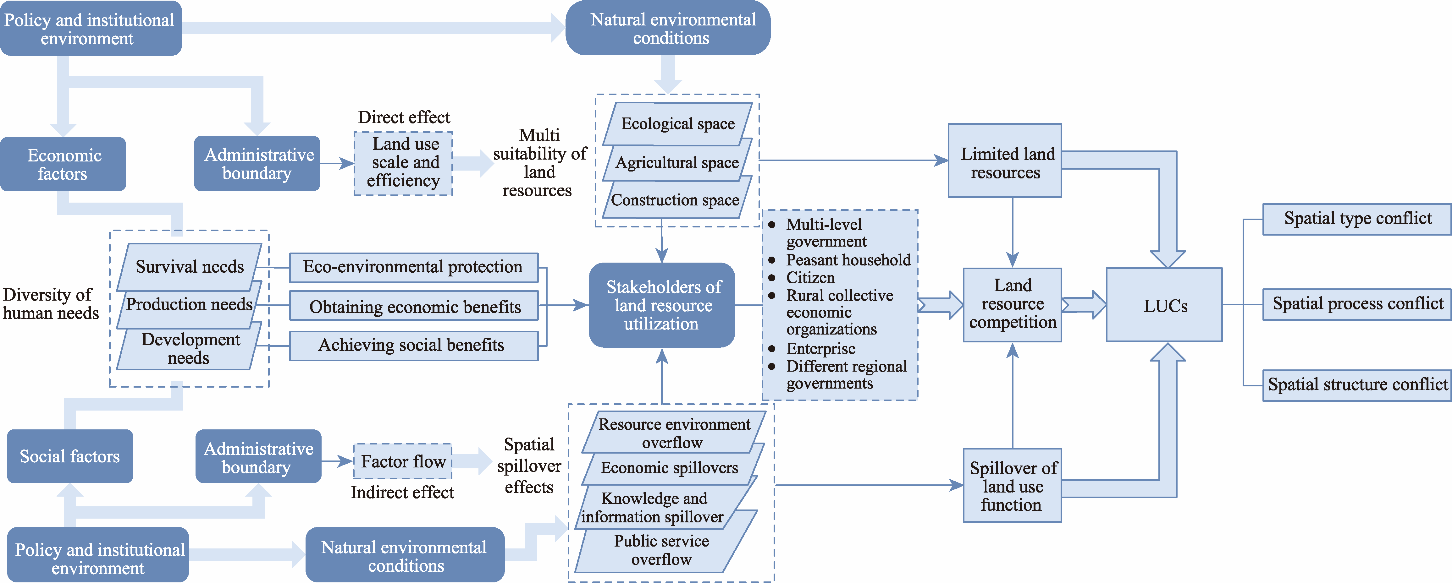
Land use conflicts (LUCs), as a spatial manifestation of the conflicts in the human-land relationships, have a profound impact on regional sustainable development. For China’s metropolitan junction areas (MJAs), the existence of “administrative district economies” has made the issue of LUCs more prominent. Based on a case study of the central Chengdu-Chongqing region, we conducted an exploratory spatial data analysis of the evolutionary process of regional LUCs. Furthermore, structural equation modeling was utilized to analyze the dynamic mechanism of LUCs in MJAs, with a particular emphasis on exploring the influences of administrative boundary. The results showed that from 2010 to 2020, LUCs in the central Chengdu-Chongqing region continued to worsen, and the spatial process conflict and spatial structure conflict indices increased by more than 30.0%. The intensification of LUCs in the central Chengdu-Chongqing region from 2010 to 2020 was mainly the result of the deterioration of conflicts in evaluation units with low conflict levels. LUCs in China’s metropolitan areas generally presented a circular gradient distribution, weakening from the core to the periphery, but there were some strong isolated conflict zones in the outer regions. LUCs in China’s MJAs were the result of interactions among multiple factors, e.g., natural environment, socio-economic development, policy and institutional processes, and administrative boundary effects. Administrative boundary affected the flow of socio-economic elements, changing the supply-and-demand competition of stakeholders for land resources, consequently exerting an indirect influence on LUCs. This study advances the theory of the dynamic mechanism of LUCs, and provides theoretical support for the governance of these conflicts in transboundary areas.
TIAN Junfeng , WANG Binyan , QIU Cheng , WANG Shijun . What are the underlying causes and dynamics of land use conflicts in metropolitan junction areas? A case study of the central Chengdu- Chongqing region in China[J]. Regional Sustainability, 2024 , 5(3) : 100161 . DOI: 10.1016/j.regsus.2024.100161
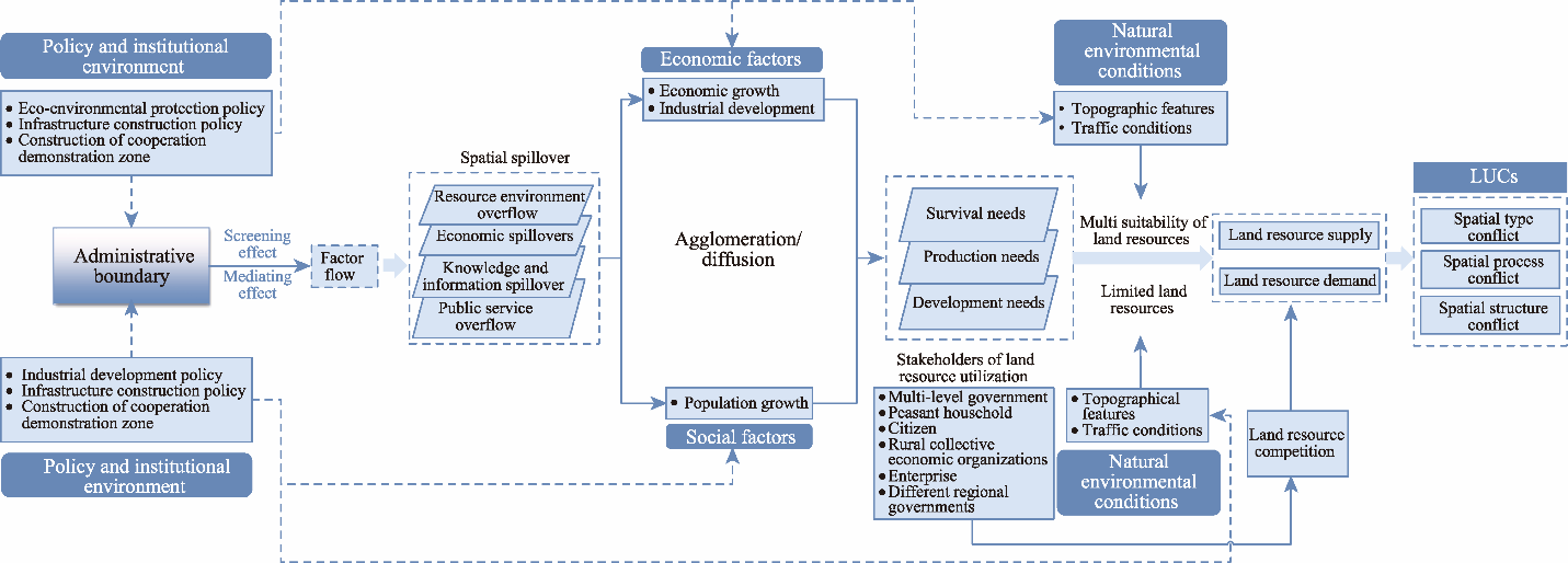
Fig. 1. Interpretation framework for land use conflicts (LUCs) in metropolitan junction areas (MJAs). |
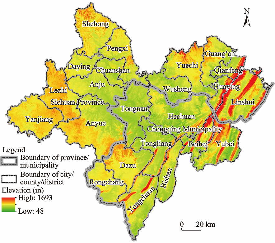
Fig. 2. Overview of the study area. Note that the figure is based on the standard map (No. GS(2024)0650) of the Map Service Center (https://www.tianditu.gov.cn/) marked by the Ministry of Natural Resources of the People’s Republic of China, and the standard map used in this study has not been modified. |
Table 1 Evaluation index of land use conflicts (LUCs) in metropolitan junction areas (MJAs). |
| Target layer | Rule layer | Index layer | Index description | Attribute | Weight |
|---|---|---|---|---|---|
| LUCs | Spatial type conflict | Development intensity index | $D I=\frac{S_{c} / S}{I}$, where DI is the construction land development intensity index; Sc is the construction space area (hm2); S is the total area of the evaluation unit (hm2); and I is the development intensity threshold of the evaluation unit. | + | 0.260 |
| Agricultural retention index | $A R=\frac{S_{a}}{G} \times 100 \%$, where AR is the agricultural retention index (%); Sa is the agricultural space area (hm2); and G is the minimum agricultural control standard values. | - | 0.032 | ||
| Spatial process conflict | Construction occupancy index | $A E C=\frac{S_{c e}+S_{a e}}{S_{a}+S_{e}}$, where AEC is the construction occupancy index; Sce is the area of ecological space occupied by construction space during 2000–2010 or 2010–2020 (hm2); Sae is the area of agricultural space occupied by construction space (hm2); Sa is the agricultural space area (hm2); and Se is the initial ecological space area (hm2). | + | 0.316 | |
| Agricultural occupancy index | $E A=\frac{S_{e a}}{S_{e}}$, where EA is the agricultural occupancy index; Sea is the area of ecological space occupied by agricultural space during 2000–2010 or 2010–2020 (hm2); and Se is the initial ecological space area (hm2). | + | 0.064 | ||
| Spatial structure conflict | Construction space fragmentation index | $I{{F}_{c}}=\frac{{{N}_{c}}}{S}$, where IFc is the spatial fragmentation index of construction space; Nc is the number of construction land patches in the evaluation unit; and S is the total area of the evaluation unit (hm2). | + | 0.128 | |
| Agricultural space fragmentation index | $I F_{a}=\frac{N_{a}}{S}$, where IFa is the spatial fragmentation index of agricultural space; Na is the number of agricultural space patches in the evaluation unit; and S is the total area of the evaluation unit (hm2). | + | 0.107 | ||
| Natural space fragmentation index | $I{{F}_{e}}=\frac{{{N}_{e}}}{S}$, where IFe is the spatial fragmentation index of natural space; Ne is the number of natural space patches in the evaluation unit; and S is the total area of the evaluation unit (hm2). | + | 0.090 |
Note: In this study, we determined I according to China’s main functional areas. The national key development zone was set to 0.30, the provincial key development zone was set to 0.25, the main agricultural product production zone was set to 0.15, and the natural function zone was set to 0.10. We determined G based on the per capita cultivated land warning line of 530 m2/person and the population size determined by the United Nations (Min et al., 2018). The symbol “+” signifies a positive correlation between the growth of this index and the occurrence of LUCs, with a negative correlation in the opposite direction. The symbol “-” indicates that the growth of this index is inversely correlated with the occurrence of LUCs. |
Table 2 Indices of the driving factors of regional LUCs. |
| Factor setting | Variable | Definition |
|---|---|---|
| Natural environmental conditions | Mean slope | Average slope per study unit (%) |
| Mean elevation | Average elevation per study unit (m) | |
| Socio-economic factors | Per capita gross domestic product (GDP) | (CNY) |
| Output value of primary industry | (CNY) | |
| Output value of secondary industry | (CNY) | |
| Output value of tertiary industry | (CNY) | |
| Population size | Population per unit (persons) | |
| Urbanization rate | Ratio of unit urban population to total population (%) | |
| Density of high-grade road | Ratio of the sum of length of unit national highway and provincial highway to unit area (km/hm2) | |
| Density of low-grade road | Ratio of the sum of length of unit county road and township road to unit area (km/hm2) | |
| Policy and institutional environment | Fixed-asset investment | Investment scale of fixed assets per unit (CNY) |
| Grain production function | Importance of food production in each unit | |
| Ecological protection function | Importance of eco-environmental protection in each unit | |
| Administrative boundary | Boundary effect |
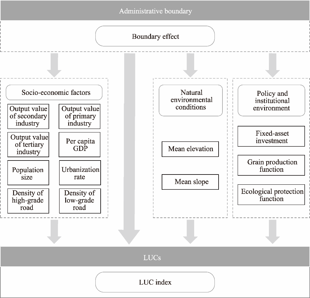
Fig. 3. Initial model of structural equation modeling (SEM). GDP, gross domestic product. |
Table 3 Main parameters used in structural equation modeling (SEM). |
| Parameter | 2010 | 2020 | Recommended value |
|---|---|---|---|
| CMIN/DF | 1.296 | 1.560 | <3.000 |
| GFI | 0.997 | 0.985 | >0.900 |
| AGFI | 0.983 | 0.966 | >0.900 |
| RMSEA | 0.032 | 0.042 | <0.080 |
Note: CMIN/DF, the ratio of chi-square to degrees of freedom; GFI, goodness-of-fit index; AGFI, adjusted goodness-of-fit index; RMSEA, root mean square error of approximation. |
Table 4 Data sources and their descriptions. |
| Data name | Data description | Data source |
|---|---|---|
| Per capita GDP | Statistical data (township as the basic unit) | Chongqing Municipal Bureau of Statistics (2022); Sichuan Provincial Bureau of Statistics (2022) |
| Output value of primary industry | ||
| Output value of secondary industry | ||
| Output value of tertiary industry | ||
| Population size | ||
| Fixed-asset investment | ||
| Land use data | Grid; 30 m×30 m | GlobeLand30 (http://www.globallandcover.com) |
| Elevation data and slope data | Grid; 90 m×90 m | Spatial information alliance (http://srtm.csi.cgiar.org/selection/inputCoord.asp) |
| Road data | Vector; line | Data Center for Resources and Environmental Sciences, Institute of Geographic Sciences and Natural Resources Research, Chinese Academy of Sciences (http://www.resdc.cn) |
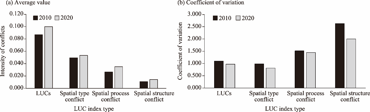
Fig. 4. Evolution of LUCs in the central Chengdu-Chongqing region in 2010 and 2020. (a), average value of LUC index; (b) coefficient of variation of LUC index. |
Table 5 Global Moran’s I of LUCs. |
| Year | Index | LUCs | STC | SPC | SSC |
|---|---|---|---|---|---|
| 2010 | Moran’s I | 0.623*** | 0.587*** | 0.614*** | 0.513*** |
| Z-value | 23.070 | 20.902 | 22.386 | 18.879 | |
| 2020 | Moran’s I | 0.616*** | 0.637*** | 0.462*** | 0.556*** |
| Z-value | 22.223 | 22.039 | 16.418 | 19.798 |
Note: Z-value, the value was obtained by dividing the Moran’s I by its standard deviation and used to determine whether the Moran’s I is significant; STC, spatial type conflict; SPC, spatial process conflict; SSC, spatial structure conflict; ***, statistical significance at the P≤0.01 level. |
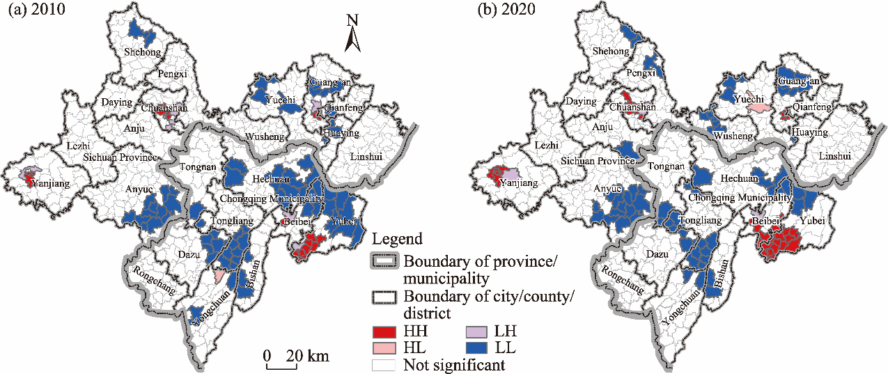
Fig. 5. Spatial agglomeration characteristics of LUCs in 2010 (a) and 2020 (b). Note that the figure is based on the standard map (No. GS(2024)0650) of the Map Service Center (https://www.tianditu.gov.cn/) marked by the Ministry of Natural Resources of the People’s Republic of China, and the standard map used in this study has not been modified. HH, the attribute values of the study region and surrounding region are both high; HL, the high-value region is surrounded by the low-value region; LH, the low-value region is surrounded by the high-value region; LL, the attribute values of the study region and surrounding region are both low. |
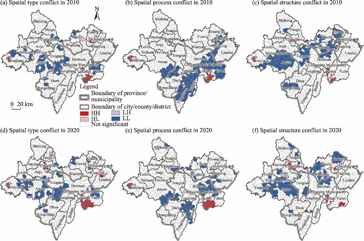
Fig. 6. Spatial agglomeration characteristics of spatial type conflict, spatial process conflict, and spatial structure conflict in 2010 and 2020. (a), spatial type conflict in 2010; (b), spatial process conflict in 2010; (c), spatial structure conflict in 2010; (d), spatial type conflict in 2020; (e), spatial process conflict in 2020; (f), spatial structure conflict in 2020. Note that the figure is based on the standard map (No. GS(2024)0650) of the Map Service Center (https://www.tianditu.gov.cn/) marked by the Ministry of Natural Resources of the People’s Republic of China, and the standard map used in this study has not been modified. |
Table 6 Regression coefficients between LUCs and influencing factors in central Chengdu-Chongqing region. |
| Variable | 2010 | 2020 |
|---|---|---|
| Output value of primary industry | -0.319*** | |
| Output value of secondary industry | 0.924*** | -0.404** |
| Output value of tertiary industry | 0.334* | |
| Per capita GDP | 0.303*** | |
| Population size | 0.433*** | |
| Fixed-asset investment | -0.268* | |
| Density of high-grade road | 0.264*** | |
| Mean slope | 0.127** | 0.176*** |
| Mean elevation | -0.208*** | -0.107* |
| Administrative boundary | -0.064 | -0.067 |
| Durbin-Watson | 1.590 | 1.317 |
| F-statistic | 23.187*** | 29.104*** |
| Adjusted R2 | 0.344 | 0.432 |
Note: Durbin-Watson is an important statistic used to test whether there is an autocorrelation (sequence correlation) phenomenon in the residual term of regression analysis. ***, statistical significance at the P≤0.01 level; **, statistical significance at the P≤0.05 level; *, statistical significance at the P≤0.10 level. |
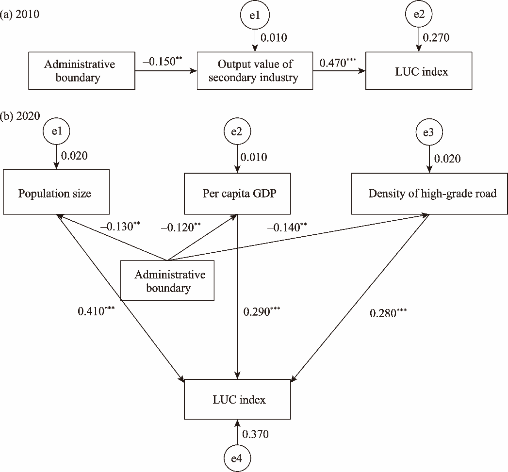
Fig. 7. SEM results of the impacts of administrative boundary on LUCs. (a), results of SEM in 2010; (b), results of SEM in 2020. In Figure 7a, e1 and e2 represent the residuals of the output value of the secondary industry and LUC index, respectively. In Figure 7b, e1, e2, e3, and e4 represent the residuals of population size, per capita GDP, the density of high-grade road, and LUC index, respectively. The value above the arrow is the regression coefficient. ** and *** indicate statistical significance at the P≤0.05 and P≤0.01 levels, respectively. |
Fig. 8. Mechanism of LUCs in the central Chengdu-Chongqing region. |
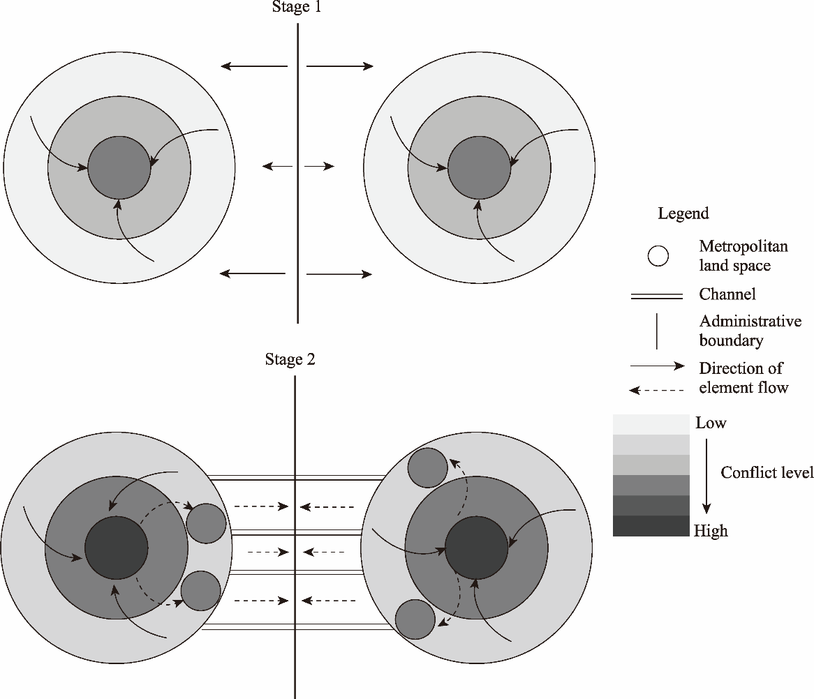
Fig. 9. Spatial evolution of LUCs in MJAs. |
| [1] |
|
| [2] |
|
| [3] |
|
| [4] |
|
| [5] |
|
| [6] |
|
| [7] |
|
| [8] |
|
| [9] |
Chongqing Municipal Bureau of Statistics, 2022. Chongqing Statistical Yearbook. Beijing: China Statistics Press (in Chinese).
|
| [10] |
|
| [11] |
|
| [12] |
|
| [13] |
|
| [14] |
|
| [15] |
|
| [16] |
|
| [17] |
|
| [18] |
|
| [19] |
|
| [20] |
|
| [21] |
|
| [22] |
|
| [23] |
|
| [24] |
|
| [25] |
|
| [26] |
|
| [27] |
|
| [28] |
|
| [29] |
|
| [30] |
|
| [31] |
|
| [32] |
|
| [33] |
|
| [34] |
Sichuan Provincial Bureau of Statistics, 2022. Sichuan Statistical Yearbook. Beijing: China Statistics Press (in Chinese).
|
| [35] |
|
| [36] |
|
| [37] |
|
| [38] |
|
| [39] |
|
| [40] |
|
| [41] |
|
| [42] |
|
| [43] |
|
| [44] |
|
| [45] |
|
| [46] |
|
| [47] |
|
| [48] |
|
| [49] |
|
| [50] |
|
| [51] |
|
| [52] |
|
| [53] |
|
/
| 〈 |
|
〉 |