Full Length Article

Green hydrogen production from wind energy in Far Eastern Federal District (FEFD), the Russian Federation

  • Mihail DEMIDIONOV , *
Expand
  • The Herzen State Pedagogical University of Russia, Saint-Petersburg, 191186, the Russian Federation
* E-mail address: (Mihail DEMIDIONOV).

Received date: 2024-07-19

  Accepted date: 2024-12-25

  Online published: 2025-08-13

Copyright

This is an open access article under the CC BY-NC-ND license (http://creativecommons.org/licenses/by-nc-nd/4.0/).

Abstract

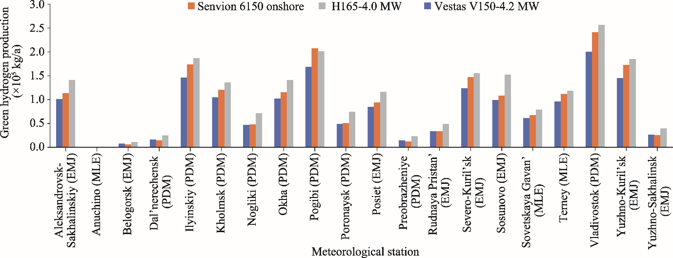
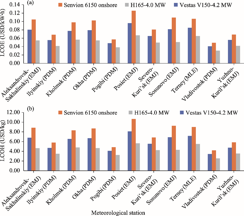
There is a gradual increase in the proportion of renewable energy sources. Green hydrogen has the potential to become one of the major energy carriers in the future. The Russian Federation, in partnership with countries in the Asia-Pacific region and especially China, has the potential to play a significant role in green hydrogen market. This study assessed the potential of developing green hydrogen energy based on wind power in the Far Eastern Federal District (FEFD) of the Russian Federation. Empirical wind speed data were collected from 20 meteorological stations in 4 regions (Sakhalinskaya Oblast’, Primorskiy Krai, Khabarovskiy Krai, and Amurskaya Oblast’) of the FEFD. The Weibull distribution was used to predict the potential of green hydrogen production. Five different methods (Empirical Method of Justus (EMJ), Empirical Method of Lysen (EML), Maximum Likelihood Method (MLE), Power Density Method (PDM), and Median and Quartiles Method (MQM)) were used to determine the parameters (scape factor and scale factor) of the Weibull distribution. We calculated the total electricity generation potential based on the technical specifications of the three wind turbines: Senvion 6150 onshore, H165-4.0 MW, and Vestas V150-4.2 MW. The results showed that Vladivostok, Pogibi, Ilyinskiy, Yuzhno-Kuril’sk, Severo-Kuril’sk, Kholmsk, and Okha stations had the higher potential of green hydrogen production, of which Vladivostok exhibited the highest potential of green hydrogen production using the wind turbine of H165-4.0 MW, up to 2.56×10⁵ kg/a. In terms of economic analysis, the levelized cost of hydrogen (LCOH) values of lower than 4.00 USD/kg were obtained at Yuzhno-Kuril’sk, Ilyinskiy, Pogibi, and Vladivostok stations using the wind turbine of H165-4.0 MW, with the values of 3.54, 3.50, 3.24, and 2.55 USD/kg, respectively. This study concluded that the FEFD possesses significant potential in the production of green hydrogen and, with appropriate investment, has the potential to become a significant hub for green hydrogen trading in the Asia-Pacific region.

Cite this article

Mihail DEMIDIONOV . Green hydrogen production from wind energy in Far Eastern Federal District (FEFD), the Russian Federation[J]. Regional Sustainability, 2025 , 6(1) : 100199 . DOI: 10.1016/j.regsus.2025.100199

1. Introduction

Since the beginning of the 20th century, renewable energy has played an increasingly significant role in the global energy mix. This process is often linked to the fourth energy transition, from traditional to renewable energy (Zhao, 2023). Despite the fact that traditional energy sources still dominate the overall system by the beginning of 2024, it is undeniable that renewable energy is experiencing significant growth. In many respects, this dynamic stems from the need for renewable energy to be integrated into the energy security strategies of various countries and regions around the world.
In the context of energy security, the development of renewable energy is driven by two key factors: the need to consistently and independently provide energy for the population, and the need to occupy a desirable market share in international energy trade. The first point is limited by the geographical distribution of renewable energy, which leads to the problem of dependence on imported raw materials in specific regions. With regard to the export component, in addition to the sale of electricity generated from renewable energy, it is essential to consider other promising energy sources. One of the sources is green hydrogen, which can be produced through electrolysis using electricity generated from renewable energy. The countries of the Asia-Pacific region are seeking to establish themselves as leaders in the global industry landscape of the 21st century (Wan et al., 2024). International cooperation at various levels is crucial for the stable development of renewable energy, including not only technological collaboration but also the establishment of a new export and import system.
Similar ideas, albeit at the strategic planning level, are outlined in the “Concept of Development of Hydrogen Energy in the Russian Federation” (The Russian Government, 2021). One of the key proposals put forward in this document is the establishment of at least three green hydrogen production clusters: the Arctic, Northwestern, and Eastern clusters. Given the increasing focus on the Russian Federation exports to the Asia-Pacific region and the strengthening of cooperation with China, it is evident that the importance of the Eastern cluster will continue to grow.
The Far Eastern Federal District (FEFD) of the Russian Federation possesses significant potential for the production of green hydrogen, primarily due to a range of natural conditions and a vast territory, which could enhance the production efficiency of renewable energy. Furthermore, the convenient geographical location of this region allows for significant reduction in the cost of green hydrogen transportation to the Asia-Pacific region. This is particularly significant, as high transportation costs remain a major obstacle to the widespread adoption of green hydrogen energy technologies. In turn, the Asia-Pacific countries, particularly China, could become key consumers of green hydrogen. For instance, Ly and Jia (2024) predicted that the sales of green hydrogen-powered vehicles in China will exceed 1.00×106 by 2035.
Wind energy is one of the main energy sources that is considered in connection with the production of green hydrogen. This topic is actively being explored in modern scientific research, and significant advancements in various aspects of wind energy have been made. For instance, Li et al. (2024a) addressed the issue of fleet optimization for offshore wind farm installations. Other issues related to maintenance and offshore wind farm operations have been actively studied (Li et al., 2024b). Therefore, any research of green hydrogen production using electricity generated from a steam generator is more or less linked to the evaluation of renewable energy potential. There is a significant body of research that utilizes multi-criteria analysis techniques, such as the Analytic Hierarchy Process (AHP), Multi-Criteria Decision Making (MCDM), and Best-Worth Method (BWM), to evaluate the potential of renewable energy in a given region (Aghaloo et al., 2023; Ahadi et al., 2023; Albraheem and AlAwlaqi, 2023; Demidionov, 2023; Raza et al., 2023). These methods allow for the consideration of a wide range of factors, including both natural and infrastructure-related ones, which is particularly important when assessing each sub-region within a larger territory. However, when analysing data from specific meteorological stations, the assessment of renewable energy potential is typically based on values related to wind speed. This approach may not fully capture the complexity and variability of conditions within a given region, as it does not account for other factors that may influence the potential of various activities.
The basis for calculating electricity production from wind energy and the subsequent production of green hydrogen is selecting model for wind speed estimation. The Weibull distribution is one of evaluation methods widely used by scholars. Furthermore, the Weibull distribution was utilized in wind speed prediction and machine learning research (Emeksiz and Tan, 2024). The use of the Weibull distribution allows for a more accurate representation of wind speed data than other statistical methods. The application of the Weibull distribution is based on the requirement to calculate two key parameters: shape factor and scale factor. These calculations are based on the collected empirical data of wind speed.
There are several methods for calculating the desired parameters. However, there is no consensus on which method is most suitable for specific regions. For instance, Nymphas and Teliat (2024) used five different approaches to analyze the wind energy potential in Nigeria. As a result, two methods yielded unsatisfactory outcomes for all meteorological stations, while the effectiveness of other methods varied depending on the region. Huo et al. (2024) employed three techniques to analyze the potential of wind energy, with the most successful outcome achieved through the use of the Maximum Likelihood Method (MLM) and Graphic Method. Kutty et al. (2024) used a total of 11 different methods to calculate various parameters in their study on the assessment of wind energy potential in Tonga. Among these methods, the best results were obtained using the Method of Moment. Koholé et al. (2023a) selected 13 different methods to evaluate the two parameters of the Weibull distribution in their assessment of solar energy potential in Cameroon. The MLM, Empirical Method of Justus (EMJ), and Empirical Method of Lysen (EML) were proved to be the effective methods in terms of their ability to provide accurate and reliable data. Additionally, it is worth mentioning the research of Aljeddani (2023) based on the data collected from certain locations in India, which found that the most accurate results were achieved through the application of the MLM. However, as noted in the aforementioned article, the Method of Moment also yielded acceptable results. Therefore, there is a need to test various techniques or methods for a specific study area.
Economic analysis is a significant aspect for analyzing the green energy potential that is also addressed in literature on similar subjects (de Almeida et al., 2024). Key metrics for economic assessment include the levelized cost of electricity (LCOE) and levelized cost of hydrogen (LCOH). There is a wide range of methods for assessing these metrics. Moreover, the values of parameters used in calculations, such as the discount rate and inflation rate, differ both across countries and over time. As a result, despite similar characteristics in terms of the potential for wind or solar power, the cost of producing one kilogram of green hydrogen may vary significantly. However, it is important to take the high costs associated with green hydrogen projects. Koholé et al. (2023b) found that the lowest cost of producing green hydrogen is approximately 4.38 USD/kg in Kousseri (Cameroon). Dabar et al. (2024) declared that the cost-effective of producing green hydrogen from wind energy (2.25 USD/kg) is better than that from solar energy (4.17 USD/kg) in the Republic of Djibouti. Juárez-Casildo et al. (2024) concluded that the use of offshore wind power leads to a decrease in the cost of green hydrogen production by up to 0.92 USD/kg compared to onshore. The study by Fetisova et al. (2017) was based on squares with a size of 1°×1° in the whole Russian Federation, using a method which reduced the accuracy of the results in determining the parameters of the Weibull distribution.
The main purpose of this study is to analyze green hydrogen production using wind energy in Sakhalinskaya Oblast’, Primorskiy Krai, Khabarovskiy Krai, and Amurskaya Oblast’ in the FEFD of the Russian Federation. The 18 selected meteorological stations are located near the coast, and another 2 meteorological stations (Belogorsk and Dal’nerechensk) are close to the boundary of the Russian Federation and China, which is particularly significant given the need for transporting the produced green hydrogen. Three different wind turbines including Senvion 6150 onshore (Rehman et al., 2024), H165-4.0 MW (The Wind Power, 2024a), and Vestas V150-4.2MW (The Wind Power, 2024b; Vestas, 2024) were used in the calculations. This study applied the economic analysis for each meteorological station using the LCOE and LCOH.
This study is the first to carry out the calculations of wind speed in Sakhalinskaya Oblast’, Primorskiy Krai, Khabarovskiy Krai, and Amurskaya Oblast’ and calculate the capacity factor based on the Weibull distribution. Moreover, this study determined the two parameters of the Weibull distribution based on five methods and assessed the accuracy of each method for each meteorological station. Finally, we calculated the data on the potential amount of green hydrogen production based on the obtained capacity factor for the first time in the study area.

2. Materials and methods

2.1. Study area

This study focuses on the four regions (Sakhalinskaya Oblast’, Primorskiy Krai, Khabarovskiy Krai, and Amurskaya Oblast’) of the FEFD, located in the southeastern part of the Russian Federation. A total of 20 meteorological stations were selected for data collection in the 4 regions (Table 1). Specifically, 18 meteorological stations are located near the coast, and some of them (such as Vladivostok) close to large port facilities and could become major hubs for international green hydrogen trade if necessary upgrades are made. Another two meteorological stations (Belogorsk and Dal’nerechensk) are close to the boundary of the Russian Federation and China. A pipeline export option is possible for green energy, but it should be noted that this mode of transportation is generally more cost-efficient for shorter distances (Berna et al., 2022). For longer distances, which are typical of the export network of the Asia-Pacific region, sea shipments currently appear to be more cost-effective.
Table 1 Description of the selected meteorological stations in the four regions.
Region Meteorological station Number Latitude (N) Longitude (E) Elevation (m)
Sakhalinskaya Oblast’ Aleksandrovsk-Sakhalinskiy 32061 50°54′ 142°10′ 31
Ilyinskiy 32121 47°59′ 142°12′ 18
Kholmsk 32133 47°03′ 142°03′ 44
Nogliki 32053 51°49′ 143°09′ 34
Okha 32010 53°35′ 142°57′ 8
Pogibi 32027 52°13′ 141°38′ 6
Poronaysk 32098 49°13′ 143°06′ 4
Severo-Kuril’sk 32215 50°41′ 156°08′ 23
Yuzhno-Kuril’sk 32165 44°01′ 145°51′ 49
Yuzhno-Sakhalinsk 32150 46°57′ 142°43′ 24
Primorskiy Krai Anuchino 31981 43°58′ 133°04′ 188
Dal’nerechensk 31873 45°56′ 133°44′ 101
Posiet 31969 42°39′ 130°48′ 36
Preobrazheniye 31989 42°54′ 133°54′ 43
Rudnaya Pristan’ 31959 44°22′ 135°51′ 34
Sosunovo 31866 46°32′ 138°20′ 4
Terney 31909 45°03′ 136°36′ 68
Vladivostok 31960 43°07′ 131°56′ 183
Khabarovskiy Kai Sovetskaya Gavan’ 31770 48°58′ 140°18′ 22
Amurskaya Oblast’ Belogorsk 31513 50°55′ 128°28′ 178

2.2. Data sources

The empirical data on the average wind speed for the 20 meteorological stations were obtained using the online weather website (http://rp5.ru/archive). This study used the data collected from 1 January in 2014 to 31 December in 2023. The wind speed at all meteorological stations was recorded at a height of 10 m above the ground level, with measurements taken every 3 hours. This study performed calculations based on the assumption that a wind turbine would be installed on a hub tower of 100 m. Therefore, it is necessary to adjust the wind speed accordingly. A simple power-low model was employed for this purpose (Shu and Jesson, 2021):
v = v R z z R α
where ν is the desired wind speed (m/s) at the height of the wind generator installation; vR is the wind speed (m/s) obtained at the meteorological station at height zR; z is the generator height above the ground level (m); and α is the power law coefficient. In this study, α value of 0.143 was selected as the most suitable option. One factor that influenced this decision was that a similar value had been used by Shu and Jesson (2021), given the relative similarities in humidity indicators and, to a certain extent, temperature conditions within the study area. Therefore, this selection appears to be justified.
The mean and maximum values, as well as standard deviation were calculated for each meteorological station. Additionally, average monthly wind speed values were calculated, along with the average values for each 3-h measurement interval to display seasonal and daily patterns in the distribution of wind speed at the elevation of 100 m.

2.3. Weibull distribution function

The Weibull distribution has been used to analyze potential wind speed and final green hydrogen production. The two parameters of the Weibull distribution: shape factor and scale factor, are shown in Equation 2. The shape factor reflects the width of the Weibull distribution (Shu and Jesson, 2021), and according to Alavi et al. (2016), the value of shape factor in most windy areas is typically between 1.200 and 2.750. However, the actual value can be significantly higher, as demonstrated by the studies of Nymphas and Teliat (2024) with the shape factor exceeding 4.000 and Yadav et al. (2024) with the shape factor of 8.920 calculated by the Method of Moment. In turn, the scale factor represents where the most of the distribution is concentrated (Ayua and Emetere, 2023). The Weibull distribution (f) was calculated as follows:
f ( v ) = k c v c k 1 exp v c k
where k is the shape factor and c is the scale factor (m/s).
The cumulative distribution function (F) can be calculated as follows:
F ( v ) = 1 exp v c k
Five different methods (EMJ, EML, MLM, Power Density Method (PDM), and Median and Quartiles Method (MQ)) were used to determine the necessary parameters of the Weibull distribution.

2.3.1. Empirical Method of Justus (EMJ) and Empirical Method of Lysen (EML)

We calculated the shape factor and scale factor of the Weibull distribution using the EMJ (Justus et al., 1978; Akpinar and Akpinar, 2009; Shu and Jesson, 2021) based on the average wind speed and standard deviation as follows:
k = σ v v ¯ 1.086
c = v ¯ Г 1 + 1 k
where σv is the standard deviation of the wind speed (m/s);
v ¯
is the mean of the wind speed (m/s); and Г is the gamma function.
In the EML (Lysen, 1983), although the difference arises at the stage of determining the scale factor, the process for determining the shape factor is similar as follows:
c = v ¯ 0.568 + 0.433 k 1 k

2.3.2. Maximum Likelihood Method (MLM)

The MLM is one of the most widely used techniques for addressing the challenge of parameter estimation in the Weibull distribution. This approach has been documented in various studies (Saleh et al., 2012; Alavi et al., 2016; Shu and Jesson, 2021; Aljeddani and Mohammed, 2023; Huo et al., 2024; Jahan et al., 2024; Kutty et al., 2024). The method is a mathematical function of wind speed, in which the shape factor and scale factor were calculated using the following equations:
k = j = 1 n v j k ln ( v j ) j = 1 n v j k j = 1 n ln ( v j ) n 1
c = 1 n j = 1 n v j k
where vj is the wind speed (m/s) measured at the time interval j and n is the number of wind speed data (>0).
In Equation 7, the shape factor appears in both sides of the equation, therefore, it cannot be solved analytically. To find the value of the shape factor using this method, an optimization technique such as the Newton-Raphson method must be employed. Ikbal et al. (2022) described a similar approach to meteorological data analysis. This method involves finding an iteration value until a convergent estimator is achieved. The Newton- Raphson method is described as follows:
k i = 1 = k i f ( k i ) f ( k i )
where i is the iteration; and f(ki) and f′(ki) are the function and its derivative, respectively, which can be calculated using the following equations:
f ( k i ) = n k n i = 1 n v i k ln ( v i ) i = 1 n v i k + i = 1 n ln ( v i )
f ( k i ) = n k n i = 1 n v i k ln ( x i ) 2 i = 1 n v i k i = 1 n v i k ln ( v i ) 2 i = 1 n v i k 2
Ikbal et al. (2022) gave the calculation equation of the convergence criterion as follows:
| k i k i = 1 | < 1.000 × 10 6
After calculating a suitable value for the shape factor, the scape factor can be determined using Equation 8.

2.3.3. Power Density Method (PDM)

The PDM is simpler to implement than the MLM. The application of this method can be found in the studies of Akdağ and Dinler (2009), Saleh et al. (2012), Soulouknga et al. (2018), and Shu and Jesson (2021). In order to determine the shape factor, the value of the Energy pattern factor (Epf) should be calculated:
E p f = v 3 ¯ ( v ¯ ) 3
where
v 3 ¯
is the mean of the sum of cubed wind speed (m/s) and
( v ¯ ) 3
is the average wind speed of the sample in a cube (m/s). The scale factor is estimated by Equation 5, and the shape factor can be calculated as follows:
k = 1 + 3.69 ( E p f ) 2

2.3.4. Median and Quartiles Method (MQM)

This method was proposed by Justus et al. (1978) based on the calculations using different quartiles of wind speed. In the study of Kutty et al. (2024), when employing the MQM, high levels of coefficient of determination (R2) were achieved in relation to the available empirical data. When applying this method, it is essential to calculate the median value of wind speed (vm), and the 25th (v0.25) and 75th (v0.75) quartiles. Then, we used the following equations to determine the shape factor and scale factor:
k = ln ln ( 0.25 ) ln ( 0.75 ) ln ( v 0.75 ) v 0.25 1.573 ln ( v 0.75 ) v 0.25
c = v m ln ( 2 ) 1 k

2.4. Goodness-of-fit test

To determine the accuracy of the model’s representation of wind speed data, given the parameters selected through various methods, it is necessary to conduct the goodness-of-fit test. Therefore, we should provide the most accurate data regarding the generation of electricity from the wind turbine to select the most accurate model for a specific meteorological station, which will provide the most accurate data of green hydrogen production. In this study, two parameters of error estimation were used: R2 and root mean square error (RMSE). As a result, a comparative analysis was conducted to determine which model provided the most accurate results in relation to the available data of meteorological stations.

2.4.1. Coefficient of determination (R2)

The R2 is a measure of the goodness-of-fit test between the observed and calculated values. It is a widely used metric in various areas, including applications of the Weibull distribution for wind speed (Huo et al., 2024). The closer the R2 is to 1.000, the more precise the resulting model is. The equation for calculating the R2 is as follows:
R 2 = 1 j = 1 m ( y j x j ) 2 j = 1 m ( y j y ¯ ) 2
where m is the total number of intervals; j is the iteration; yj is the frequency of empirical wind speed data; xj is the frequency distribution of wind speed data calculated with the Weibull distribution; and
y ¯
is the mean of the frequency of empirical wind speed data.

2.4.2. Root mean square error (RMSE)

The RMSE is a performance metric that measures the average squared difference between observed and calculated values. A lower RMSE value indicates a better fit of a model to observed values. The RMSE is expressed in the same units as the target value. The following equation is employed to compute the RMSE:
RMSE = j = 1 m ( y j x j ) 2 m

2.5. Electricity and green hydrogen production

In the final stage, it will be necessary to calculate the potential amount of energy that can be generated using a wind turbine, and as a result, the quantity of green hydrogen can be produced. The key factor for calculating the efficiency of a wind turbine is the capacity factor, which represents the ratio of the output power (Pout) to the rated power of the wind turbine, over a specified time period. We calculated the capacity factor based on the shape factor and scale factor. The equation for calculating the capacity factor (Cf) is as follows (Adaramola et al., 2014):
C f = exp v c c k exp v r c k v r c k v c c k exp v f c k
where vc is the cut-in wind speed (m/s); vr is the rated wind speed (m/s); and vf is the cut-out wind speed (m/s). In the next step, the annual electricity generation using the wind turbine can be calculated (Ashrafi et al., 2018):
E out = C f × P rated × 8760
where Eout is the electricity generation (kW•h) and Prated is the wind turbine rated power (kW•h). A system for generating green hydrogen using wind power typically comprises the following components: wind turbine, control system, rectifier, and electrolyzer (Alavi et al., 2016; Ashrafi et al., 2018). In this study, a decision was made to select an alkaline electrolyzer. The choice is justified by the fact that the alkaline electrolyzer is currently more cost-effective than the Proton exchange membrane (PEM) (Hesty et al., 2024). As the final product of the process is green hydrogen, which has a high cost of transportation, it is essential to consider cost saving opportunities at various production stages. In order to calculate the annual green hydrogen production capacity based on the electricity generated, it is essential to determine the certain parameters of the wind turbine. It is also worth noting that the alkaline electrolyzer is technically simpler than the PEM or solid oxide (David et al., 2019).
In order to calculate the potential amount of green hydrogen production, it is necessary to define the parameters of the electrolysis process. The first parameter is the efficiency of the rectification process (ηconv). In various studies, the efficiency value of the rectification process ranges from 75.0% to 95.0%. For the current study, the value of 75.0% was employed. The second factor is the power consumption of the electrolyzer (ECel), ranging from 5.00 to 6.00 kW•h/m3. The following equation is used to calculate the amount of produced green hydrogen (Ashrafi et al., 2018):
M H 2 = E out η conv EC el
where MH2 is the mass of green hydrogen (m3); ηconv is the efficiency of the rectification process (%); and ECel is the power consumption of the electrolyzer (kW•h/m3). Specifically, 1 kg of green hydrogen is equal to 11.13 m3, therefore, in order to convert the amount of green hydrogen produced into kilogram (kg), it is necessary to multiply the value of 11.13 m3.

2.6. Economic feasibility

To assess the economic feasibility of green energy, it is essential to calculate the indicators that characterize the costs of both electricity generation and green hydrogen production. In contemporary scientific research, some of the most commonly used indicators include the LCOE and LCOH.
The LCOE was calculated by the following equation (Rezaei et al., 2020):
LCOE = C ini + h = 1 N C om 1 + f 1 + r h h = 1 N E out ( 1 + d ) h
where LCOE is the levelized cost of electricity (USD/kW•h); Cini is the investment cost of the wind turbine (USD); Com is the operation-maintenance cost (USD); r is the discount rate (%); d is the degradation rate (%); f is the inflation rate (%); N is the turbine lifespan (a); and h is the year (a).
The cost of green hydrogen production will depend on two main factors (Dehshiri et al., 2024): the cost of the electricity supplied (Celectricity) and the cost of the electrolysis process (Celectrolyzer). These two factors were calculated as follows:
C electricity = LCOE i = 1 N E out N
C electrolyzer = C u.electrolyzer × M H 2 × EC el t × 8760 × С f × η conv
where Cu.electrolyzer is the electrolyzer unit price (USD) and t is the electrolyzer lifespan (a).
Finally, the LCOH was calculated by the following equation:
LCOH = C electricity + C electrolyzer M H 2
where LCOH is the levelized cost of hydrogen (USD/kg).

2.7. Assumptions and limitation of research

This study made some assumptions that are often not precisely defined and may vary in different years, studies, and countries. These assumptions include: the wind turbine price was taken as 1000.00 USD/kW of nominal power; the cost of turbine installation was assumed to be 40.0% of capital investment (Rezaei et al., 2020; Dehshiri et al., 2024); the electrolyzer unit price was taken as 1000.00 USD/kW with the lifetime of 7 a; and the discount and inflation rates were taken as 8.0% and 8.5%, respectively.

3. Results and discussion

3.1. Wind speed change characteristics

Tables 2 and 3 present the statistics related to the annual and monthly wind speed at 20 meteorological stations during 2014-2023, respectively.
Table 2 Annual wind speed statistics of 20 meteorological stations during 2014-2023.
Meteorological station Average wind speed (m/s) Standard deviation (m/s) Maximum wind speed (m/s) Median wind speed (m/s)
Aleksandrovsk-Sakhalinskiy 5.172 2.489 21.371 4.517
Anuchino 2.037 0.752 5.734 1.911
Belogorsk 2.415 1.186 10.946 2.259
Dal’nerechensk 3.049 1.377 10.251 2.954
Ilyinskiy 6.220 3.145 25.888 5.560
Kholmsk 5.045 2.831 19.112 4.517
Nogliki 4.289 1.749 15.984 3.996
Okha 5.360 2.557 21.371 4.865
Pogibi 6.468 3.690 25.019 5.560
Poronaysk 4.318 1.808 15.463 3.996
Posiet 4.588 2.446 19.459 3.822
Preobrazheniye 3.137 1.266 14.247 2.954
Rudnaya Pristan’ 3.358 1.773 15.637 2.954
Severo-Kuril’sk 5.145 3.133 21.197 4.517
Sosunovo 5.700 2.226 22.587 5.386
Sovetskaya Gavan’ 3.525 2.572 22.934 2.780
Terney 4.273 3.057 21.197 3.300
Vladivostok 7.843 3.120 23.455 7.297
Yuzhno-Kuril’sk 5.842 3.093 24.845 5.212
Yuzhno-Sakhalinsk 3.293 1.611 12.857 2.954
Table 3 Average monthly wind speed of 20 meteorological stations.
Meteorological station Average monthly wind speed (m/s)
January February March April May June July August September October November December
Aleksandrovsk-Sakhalinskiy 5.308 5.369 5.318 5.299 4.721 3.897 3.794 4.033 5.128 6.099 6.709 6.419
Anuchino 1.853 2.104 2.369 2.708 2.403 1.823 1.693 1.545 1.779 2.236 1.996 1.905
Belogorsk 1.817 2.095 2.766 3.602 3.140 2.254 2.133 1.908 2.183 2.582 2.387 1.979
Dal’nerechensk 2.844 3.190 3.489 3.997 3.496 2.711 2.499 2.243 2.452 3.401 3.274 2.987
Ilyinskiy 6.150 6.104 6.295 6.709 6.004 5.470 5.115 5.343 5.693 6.821 7.429 7.492
Kholmsk 5.152 5.376 5.426 5.631 4.774 3.550 3.498 3.854 4.724 5.858 6.366 6.293
Nogliki 4.331 4.451 4.323 4.933 4.482 4.035 3.699 3.710 3.910 4.362 4.521 4.731
Okha 6.097 5.622 4.997 5.610 5.152 4.676 4.707 4.409 4.492 5.320 6.248 7.202
Pogibi 6.061 5.786 5.292 5.931 6.206 6.869 7.429 6.255 6.486 7.180 6.826 6.949
Poronaysk 4.334 4.333 4.383 4.572 4.505 3.912 3.744 4.090 4.319 4.653 4.454 4.508
Posiet 6.161 5.445 4.619 4.510 4.099 3.585 3.232 3.741 3.635 4.345 5.422 6.296
Preobrazheniye 3.628 3.190 2.981 3.082 2.941 2.710 2.513 3.101 3.489 3.298 3.320 3.388
Rudnaya Pristan’ 5.139 4.428 3.396 3.264 2.830 2.248 2.040 2.316 2.721 3.474 3.797 4.698
Severo-Kuril’sk 6.602 7.027 6.760 6.200 4.360 3.362 2.921 3.315 4.429 5.474 5.577 5.884
Sosunovo 6.634 6.259 5.654 5.753 5.655 5.314 4.537 5.008 5.436 5.688 5.849 6.667
Sovetskaya Gavan’ 3.937 3.536 3.524 3.804 3.192 2.380 2.002 2.309 3.139 4.578 4.870 5.029
Terney 7.696 6.410 4.497 3.947 2.961 1.695 1.439 1.851 2.504 4.547 6.057 7.738
Vladivostok 8.414 7.977 7.824 8.293 8.154 7.651 7.011 7.362 7.147 7.910 8.144 8.105
Yuzhno-Kuril’sk 7.098 6.903 6.356 5.977 4.822 4.641 3.646 4.167 4.551 6.371 7.031 7.271
Yuzhno-Sakhalinsk 3.152 3.176 3.419 3.841 4.100 4.003 3.340 3.038 2.741 3.074 2.829 2.811
There was a significant variation in the average wind speed of 20 meteorological stations. The minimum value of the annual average wind speed was found in Anuchino (2.037 m/s), while the maximum value appeared in Vladivostok (7.843 m/s). Vladivostok was characterized by the high values of the standard deviation and median wind speed. Meteorological stations located in Sakhalinskaya Oblast’ had the highest average wind speed, with Vladivostok being a notable exception. It was worth noting that at most meteorological stations, the highest wind speed was typically recorded during the winter season (December to February of the next year). However, it should also be noted that Vladivostok had the advantage of high wind speed stability throughout the year. In addition, the average wind speed of Vladivostok was the highest and it belonged to the 7th class of wind power according to the classification system presented in the study of Jahan et al. (2024).
The strongest wind speed was typically observed in the daytime, between 11:00 and 20:00 (LST) at almost all monitored meteorological stations (Fig. 1). The only exception was Preobrazheniye located in Primorskiy Krai.
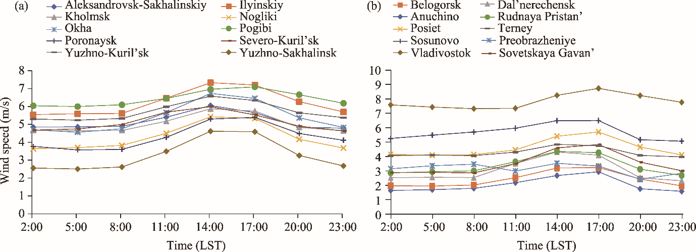
Fig. 1. Wind speed of meteorological stations in Sakhalinskaya oblast’ (a) and Primorskiy Krai, Amurskaya oblast’, and Khabarovskiy Krai (b).
From Tables 2 and 3 we can see that there were some meteorological stations where the generation of significant amounts of electricity through wind power was unlikely due to the extremely low average wind speed, such as Anuchino, Dal’nerechensk, and Preobrazheniye.

3.2. Weibull distribution characteristics

We calculated the shape factor and scale factor of the Weibull distribution based on five methods (Table 4). The shape factor values varied from 1.301 to 3.560 at all meteorological stations for all methods. The scale factor values changed from 2.118 to 8.834. Similarly, Alavi et al. (2016) showed that the shape factor varied to a lesser extent than the scale factor, which was consistent with our expectations. A comparison between the empirical wind speed data and the wind speed data calculated by the five methods is presented in Figure 2. Additionally, Vladivostok, Pogibi, and Ilyinskiy stations observed the relatively high wind speeds (Fig. 2).
Table 4 Shape factor and scale factor values calculated using five methods at the 20 meteorological stations.
Meteorological station EMJ EML MLE PDM MQM
Shape factor Scale factor Shape factor Scale
factor
Shape factor Scale
factor
Shape factor Scale
factor
Shape factor Scale factor
Aleksandrovsk-Sakhalinskiy 2.210 5.840 2.210 5.842 2.192 5.857 2.045 5.582 2.676 5.180
Anuchino 2.951 2.283 2.951 2.282 2.862 2.283 2.776 2.299 3.560 2.118
Belogorsk 2.166 2.727 2.166 2.728 2.149 2.731 2.088 2.715 2.269 2.655
Dal’nerechensk 2.371 3.440 2.371 3.441 2.351 3.446 2.291 3.391 2.595 3.402
Ilyinskiy 2.097 7.022 2.097 7.026 2.109 7.050 2.023 6.646 2.132 6.602
Kholmsk 1.873 5.682 1.873 5.686 1.901 5.713 1.822 5.453 1.765 5.560
Nogliki 2.650 4.826 2.650 4.827 2.516 4.829 2.423 4.681 3.298 4.466
Okha 2.234 6.052 2.234 6.054 2.220 6.068 2.127 5.774 2.355 5.684
Pogibi 1.840 7.280 1.840 7.285 1.884 7.331 1.748 6.898 2.016 6.668
Poronaysk 2.573 4.863 2.573 4.863 2.477 4.870 2.376 4.710 3.114 4.496
Posiet 1.980 5.176 1.980 5.179 2.012 5.207 1.840 4.985 2.487 4.430
Preobrazheniye 2.679 3.528 2.679 3.529 2.572 3.529 2.505 3.485 2.990 3.339
Rudnaya Pristan’ 2.001 3.789 2.001 3.791 2.021 3.807 1.826 3.715 2.757 3.374
Severo-Kuril’sk 1.714 5.770 1.714 5.774 1.749 5.810 1.650 5.557 1.765 5.560
Sosunovo 2.776 6.404 2.776 6.404 2.612 6.403 2.538 6.122 3.240 6.031
Sovetskaya Gavan’ 1.409 3.872 1.409 3.875 1.538 3.954 1.301 3.892 1.916 3.366
Terney 1.438 4.707 1.438 4.711 1.491 4.761 1.416 4.667 1.394 4.294
Vladivostok 2.721 8.817 2.721 8.818 2.657 8.834 2.576 8.290 2.904 8.279
Yuzhno-Kuril’sk 1.995 6.591 1.995 6.595 2.014 6.621 1.879 6.263 2.269 6.126
Yuzhno-Sakhalinsk 2.170 3.718 2.170 3.720 2.163 3.730 2.029 3.647 2.418 3.437

Note: EMJ, Empirical Method of Justus; EML, Empirical Method of Lysen; MLE, Maximum Likelihood Method; PDM, Power Density Method; MQM, Median and Quartiles Method.

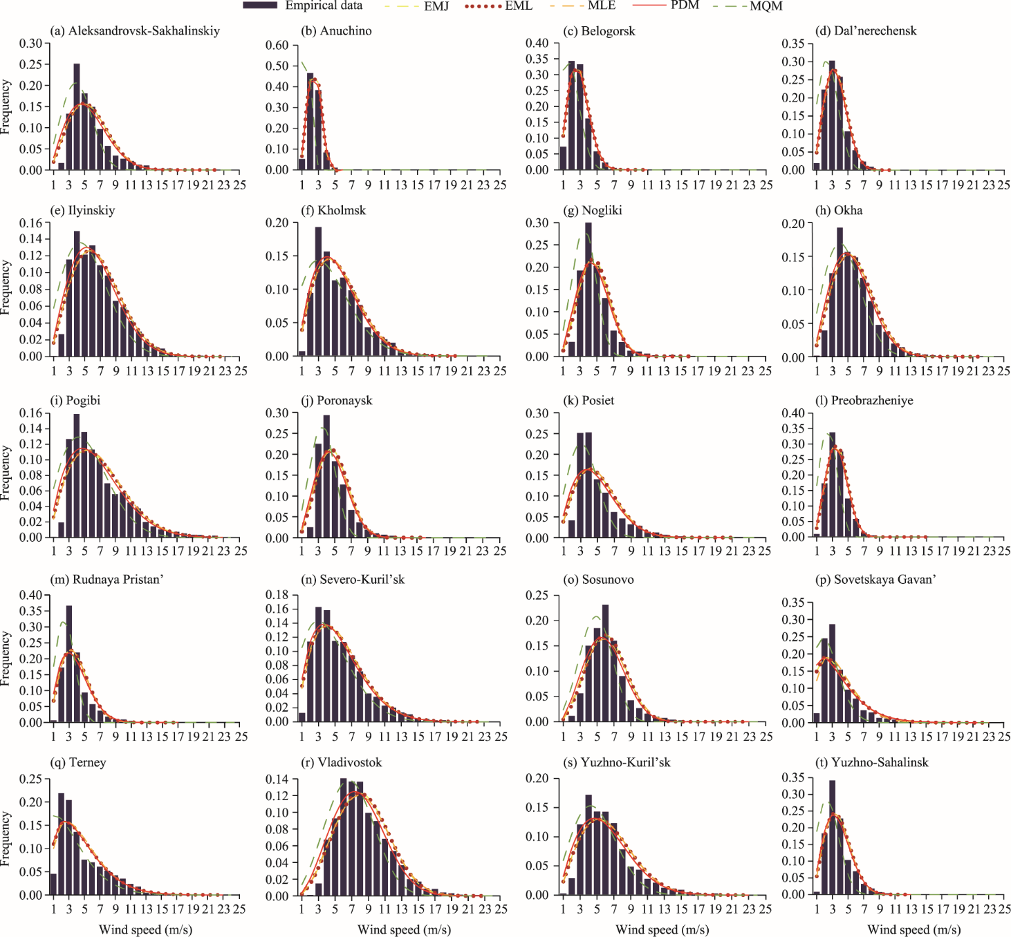
Fig. 2. Histogram of empirical wind speed data and the Weibull distribution of wind speed data calculated by the five methods (Empirical Method of Justus (EMJ), Empirical Method of Lysen (EML), Maximum Likelihood Method (MLE), Power Density Method (PDM), and Median and Quartiles Method (MQM)) at the 20 meteorological stations (a-t).
It was also worth considering which methods yielded the most accurate results in comparison to the empirical wind speed data at meteorological stations. The goodness-of-fit test results are shown in Table 5. The efficiency of a particular method was contingent with the specific meteorological station. In general, the uses of EMJ, EML, MLE, and PDM allowed to achieve a high degree of similarity with the distribution of empirical wind speed data. Only the MQM yielded extremely suboptimal results. In most cases, the efficiency of EML was slightly superior to that of EMJ. However, overall, the outcomes of employing these methods were nearly identical. The similarity in the performances of the EML, EMJ, and MLE were also noted in the study of Kutty et al. (2024). The PDM has also demonstrated high performance in goodness-of-fit test, despite the fact that it was, for example, inferior to the EML and EMJ (Kang et al., 2021).
Table 5 Goodness-of-fit test results of the five methods.
Meteorological station EMJ EML MLE PDM MQM
R2 RMSE R2 RMSE R2 RMSE R2 RMSE R2 RMSE
Aleksandrovsk-Sakhalinskiy 0.8479* 0.0280* 0.8477 0.0280 0.8454 0.0283 0.8476 0.0281 0.7597 0.0351
Anuchino 0.9857 0.0223 0.9857 0.0223 0.9876* 0.0216* 0.9858 0.0249 0.0821 0.2455
Belogorsk 0.9773* 0.0202* 0.9772 0.0202* 0.9762 0.0208 0.9729 0.0225 0.5375 0.0919
Dal’nerechensk 0.9691 0.0203 0.9690 0.0204 0.9683 0.0208 0.9724* 0.0198* 0.6589 0.0680
Ilyinskiy 0.9408 0.0121 0.9406 0.0121 0.9391 0.0123 0.9487* 0.0112* 0.8401 0.0200
Kholmsk 0.9090 0.0176 0.9088 0.0177 0.9057 0.0179 0.9160* 0.0168* 0.7595 0.0286
Nogliki 0.8929 0.0313* 0.8929 0.0313* 0.8886 0.0326 0.8972* 0.0316 0.7365 0.0499
Okha 0.9476 0.0143 0.9475 0.0143 0.9466 0.0145 0.9528* 0.0136* 0.8178 0.0263
Pogibi 0.8682 0.0180 0.8680 0.0180 0.8656 0.0181 0.8689* 0.0177* 0.7981 0.0220
Poronaysk 0.8614 0.0345 0.8613 0.0345 0.8603 0.0351 0.8742* 0.0336* 0.7416 0.0479
Posiet 0.7893* 0.0358* 0.7890 0.0358 0.7879 0.0358 0.7828 0.0363 0.6852 0.0443
Preobrazheniye 0.9724 0.0184* 0.9724 0.0184* 0.9719 0.0193 0.9743* 0.0188 0.6065 0.0733
Rudnaya Pristan’ 0.8431* 0.0412 0.8428 0.0412 0.8430 0.0411* 0.8176 0.0444 0.6531 0.0627
Severo-Kuril’sk 0.9414* 0.0126* 0.9413 0.0127 0.9407 0.0126* 0.9383 0.0128 0.8181 0.0220
Sosunovo 0.9288* 0.0189* 0.9288* 0.0189* 0.9183 0.0208 0.9243 0.0198 0.8277 0.0286
Sovetskaya Gavan’ 0.7853 0.0366 0.7853 0.0366 0.8319* 0.0328* 0.7280 0.0409 0.6796 0.0460
Terney 0.8469 0.0243 0.8468 0.0243 0.8474* 0.0242* 0.8451 0.0244 0.7229 0.0331
Vladivostok 0.9390 0.0122 0.9389 0.0122 0.9394 0.0123 0.9549* 0.0105* 0.8624 0.0176
Yuzhno-Kuril’sk 0.9187* 0.0159* 0.9185 0.0159* 0.9180 0.0159* 0.9137 0.0161 0.8457 0.0212
Yuzhno-Sakhalinsk 0.8970* 0.0353* 0.8968 0.0354 0.8950 0.0358 0.8923 0.0367 0.6049 0.0691

Note: * means the highest similarity degree with the empirical data; R2, coefficient of determination; RMSE, root mean square error.

3.3. Electricity generation and green hydrogen production

The three wind turbines (Senvion 6150 onshore, H165-4.0 MW, and Vestas V150-4.2MW) were used to calculate the capacity factor, annual electricity generation values, and the potential amount of green hydrogen that could be produced. The technical specifications of the wind turbines required for the calculations are provided in Table 6. The capacity factor values ranged from very low (0.000) at Anuchino station to extremely high (0.554) at Vladivostok station (Fig. 3).
Table 6 Technical specifications of the three wind turbines.
Wind turbine Lifetime (a) Rated power (×106 W) Cut-in wind speed (m/s) Rated wind speed (m/s) Cut-off wind speed (m/s)
Senvion 6150 onshore 20 6.15 3.500 12.000 25.000
H165-4.0 MW 20 4.00 3.000 9.100 20.000
Vestas V150-4.2 MW 20 4.20 3.000 11.000 24.500
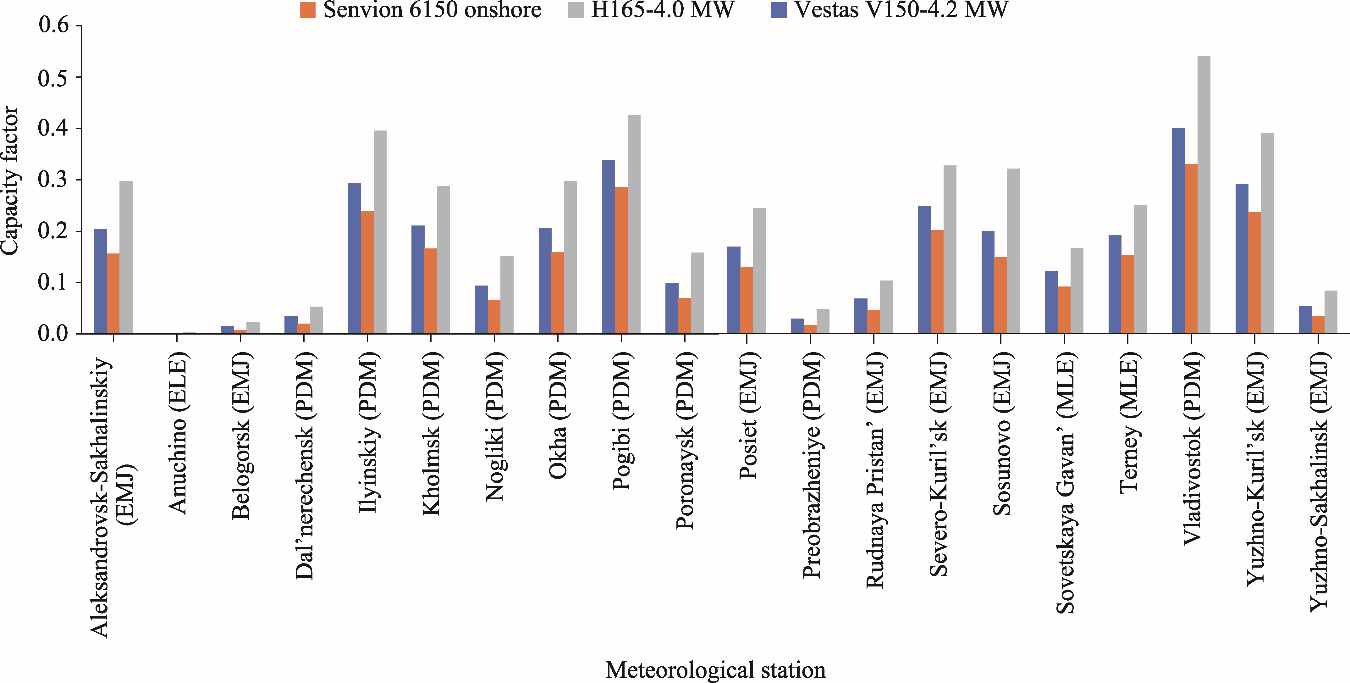
Fig. 3. Capacity factor of the three wind turbines at 20 meteorological stations. The calculated methods are specified in parentheses.
The values were calculated separately for each meteorological station using the method that demonstrated the best performance in the goodness-of-fit test. The capacity factor value above 0.500 was achieved at Vladivostok station using the H165 wind turbine. The higher capacity factor values (0.400-0.500) can be seen at Pogibi station (by H165-4.0 MW), Vladivostok (by Vestas V150-4.2MW), and Ilyinskiy (by H165-4.0 MW) stations. The extremely low capacity factor values were recorded at Anuchino, Belogorsk, and Preobrazheniye stations.
Some meteorological stations exhibited particularly high-performance values of electricity generation and potential green hydrogen production. The highest levels of electricity generation were found by Senvion 6150 onshore and H165-4.0 MW (Fig. 4). Vladivostok, Pogibi, Ilyinskiy, Yuzhno-Kuril’sk, Severo-Kuril’sk, Kholmsk, and Okha stations had the higher potential of green hydrogen production, with values of 2.56×10⁵, 2.05×10⁵, 1.87×10⁵, 1.84×10⁵, 1.60×10⁵, 1.36×10⁵, and 1.40×10⁵ kg/a, respectively (Fig. 5). At the same time, most of meteorological stations had the better performance in green hydrogen production by H165-4.0 MW. However, for some meteorological stations, Senvion 6150 onshore was not significantly ahead. This is because the latter can operate at higher wind speed, which was significant for meteorological stations with specific characteristics, such as Vladivostok. Nevertheless, the lower rated speed of H165-4.0 MW compared to Vestas V150 MW and Senvion 6150 onshore allowed it to maintain a high position in terms of both electricity generation and the capacity factor. The high rated power value of Senvion 6150 onshore gave it a competitive advantage in terms of electricity generation. However, it fell behind in terms of the capacity factor in comparison to other wind turbines.
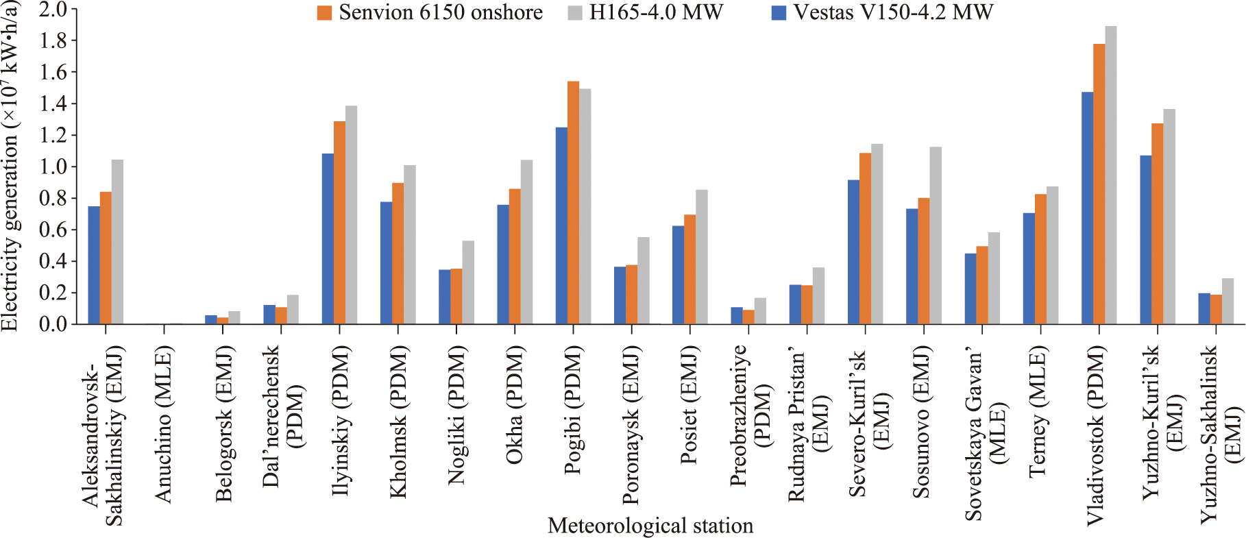
Fig. 4. Annual electricity generation by the three wind turbines at 20 meteorological stations. The calculated methods are specified in parentheses.
Fig. 5. Annual green hydrogen production by the three wind turbines at 20 meteorological stations. The calculated methods are specified in parentheses.
The results of the economic indicators are presented in Figure 6, which showed the data only for those meteorological stations where the LCOE was less than 0.10 USD/kW•h for at least one of the wind turbines. Other meteorological stations with higher economic indicators were excluded as they were not economically viable. Although Senvion 6150 onshore may be competitive with H165-4.0 MW in terms of overall electricity generation at certain meteorological stations, the LCOE and LCOH by Senvion 6150 onshore were too high. This is due to the high rated power of Senvion 6150 onshore, which has resulted in both high capital investment costs and high annual maintenance expenses. However, the ability of Senvion 6150 onshore to operate at higher wind speed was not a significant factor for the selected meteorological stations. Certain meteorological stations had promising economic indicators. For instance, Yuzhno-Kuril’sk, Ilyinskiy, Pogibi, and Vladivostok obtained the LCOH values of 3.54, 3.50, 3.24, and 2.55 USD/kg, respectively, using the wind turbine of H165-4.0 MW. These LCOH values were in line with those obtained in recent studies (Ahshan et al., 2022; Dabar et al., 2024; Schmidhalter et al., 2024). However, electrolyzer efficiency was assumed to be 75.0%, which was near the minimum threshold. Also, the subsequent costs of green hydrogen transportation were an area of interest, which remained a significant challenge for the large-scale adoption of green hydrogen energy.
Fig. 6. Levelized cost of electricity (LCOE) and levelized cost of hydrogen (LCOH) for the three wind turbines. Note that only meteorological stations where the LCOE was less than 0.10 USD/kW•h for at least one of the wind turbines are shown. The calculated methods are specified in parentheses.
In general, there is a significant potential for the production of green hydrogen in the study area using electricity generated in a wind farm. This is particularly true for Sakhalin Island and the southern part of Primorskiy Krai. It is advisable to consider precisely those areas with wind speeds consistently high throughout the year. For example, Vladivostok, which also has an advantage of developed port infrastructure with necessary modernization, could be adapted for green hydrogen trade. This could have positive economic implications given the size of the Asia-Pacific region market.
At the same time, the issue of economic viability remains significant. From this perspective, the more significant indicator is not the exact potential amount of green hydrogen production, but rather the capacity factor of meteorological station. This is because wind turbines may vary in terms of their specifications and characteristics, but the capacity factor will be consistent within a given region over an extended period. According to Adaramola et al. (2011), investments in wind turbines become effective when the capacity factor exceeds 0.250. This study has identified a number of meteorological stations where this practice was followed.
In regards to the selection of wind turbines, this study found that H165-4.0 MW demonstrated superior performance in terms of both the capacity factor and economic efficiency. This can be attributed to the relatively low rated wind speed of this turbine. Despite Senvion 6150 onshore indicated a higher rated power of 6.15×10⁶ W, H165-4.0 MW and Vestas V150-4.2 MW showed more promising results.

4. Conclusions

This study attempted to explore the potential of four regions (Sakhalinskaya Oblast’, Primorskiy Krai, Khabarovskiy Krai, and Amurskaya Oblast’) in the FEFD to produce green hydrogen through the use of wind energy. Based on the data from 20 meteorological stations during 2014-2023, we performed a statistical analysis and calculated two parameters (shape factor and scale factor) of the Weibull distribution using five different methods (EMJ, EML, MLE, PDM, and MQ).
The results indicated that the most suitable methods for the study area are the EMJ, EML, MLE, and PDM. At most meteorological stations, these four methods yielded relatively similar results with the empirical data, while the MQM produced results that were significantly different from the empirical data. Additionally, Vladivostok, Pogibi, Ilyinskiy, Yuzhno-Kuril’sk, Severo-Kuril’sk, Kholmsk, and Okha stations had the higher potential of green hydrogen production, with values of 2.56×10⁵, 2.05×10⁵, 1.87×10⁵, 1.84×10⁵, 1.60×10⁵, 1.36×10⁵, and 1.40×10⁵ kg/a, respectively. An economic analysis was also conducted, which resulted in the LCOH values of Yuzhno-Kuril’sk, Ilyinskiy, Pogibi, and Vladivostok stations below 4.00 USD/kg using the wind turbine of H165-4.0 MW. However, the calculations of the LCOE and LCOH may not always produce accurate values due to uncertainty and constant changes in certain indicators that taken into account in the calculations, such as the inflation rate and discount rate.
Given the favourable location of the study area for trade, there is a significant number of regions that need to be explored the potential green hydrogen production. An important aspect for research in this area is the analysis of various methods for producing green hydrogen. It would also be beneficial to examine the potential use of solar energy and hydroelectric power for generating green hydrogen, or even a combined system, such as wind-solar power. Additionally, analyzing the potential for using offshore wind farms in the electrolysis process, particularly in the areas near Sakhalin Island, could also be worthwhile. Another field of significant research is the use of various types of electrolysis systems, such as Alkaline and PEM, and the calculation of their performance based on the data obtained from the current study. It is also essential to address the issue of reducing CO2 emissions, which is particularly significant given the high reliance of the FEFD on thermal power generation.

Authorship contribution statement

Mihail DEMIDIONOV: data curation, writing - original draft, formal analysis, writing - review & editing, conceptualization, methodology, and project administration. The author approved the manuscript.

Declaration of conflict of interest

The authors declare that he has no known competing financial interests or personal relationships that could have appeared to influence the work reported in this paper.

Acknowledgements

The author would like to express his gratitude to Prof. Yuri GLADKIY for invaluable guidance and collaboration.
[1]
Adaramola M., Paul S., Oyedepo S.O., 2011. Assessment of electricity generation and energy cost of wind energy conversion systems in North-Central Nigeria. Energy Conv. Manag. 52, 3363-3368.

[2]
Adaramola M.S., Agelin-Chaab M., Paul S.S., 2014. Analysis of hybrid energy systems for application in southern Ghana. Energy Conv. Manag. 88, 284-295.

[3]
Aghaloo K., Ali T., Chiu, Y-R., et al., 2023. Optimal site selection for the solar-wind hybrid renewable energy systems in Bangladesh using an integrated GIS-based BWM-fuzzy logic method. Energy Conv. Manag. 283, 116899, doi: 10.1016/j.enconman.2023.116899.

[4]
Ahadi P., Fakhrabadi F., Pourshaghaghy A., et al., 2023. Optimal site selection for a solar power plant in Iran via the Analytic Hierarchy Process (AHP). Renew. Energy. 215, 118944, doi: 10.1016/j.renene.2023.118944.

[5]
Ahshan R., Onen A., Al-Badi A.H., 2022. Assessment of wind-to-hydrogen (wind-H2) generation prospects in the Sultanate of Oman. Renew. Energy. 200, 271-282.

[6]
Akdağ S.A., Dinler A., 2009. A new method to estimate Weibull parameters for wind energy applications. Energy Conv. Manag. 50(7), 1761-1766.

[7]
Akpinar S., Akpinar E.K., 2009. Estimation of wind energy potential using finite mixture distribution models. Energy Conv. Manag. 50(4), 877-884.

[8]
Alavi O., Mostafaeipour A., Qolipour M., 2016. Analysis of hydrogen production from wind energy in the southeast of Iran. Int. J. Hydrogen Energy. 41(34), 15158-15171.

[9]
Albraheem L., AlAwlaqi L., 2023. Geospatial analysis of wind energy plant in Saudi Arabia using a GIS-AHP technique. Energy Rep. 9, 5878-5898.

[10]
Aljeddani S.M.A., Mohammed M.A., 2023. A novel approach to Weibull distribution for the assessment of wind energy speed. Alex. Eng. J. 78, 56-64.

[11]
Ashrafi Z.N., Ghasemian M., Shahrestani M.I., et al., 2018. Evaluation of hydrogen production from harvesting wind energy at high altitudes in Iran by three extrapolating Weibull methods. Int. J. Hydrogen Energy. 43(6), 3110-3132.

[12]
Ayua T.J., Emetere M.E., 2023. Technical analysis of wind energy potentials using a modified Weibull and Raleigh distribution model parameters approach in the Gambia. Heliyon. 9(9), e20315, doi: 10.1016/j.heliyon.2023.e20315.

[13]
Berna C., Vargas-Salgado C., Alfonso-Solar D., et al., 2022. Hydrogen production from surplus electricity generated by an autonomous renewable system: Scenario 2040 on Grand Canary Island, Spain. Sustainability. 14(19), 11884, doi: 10.3390/su141911884.

[14]
Dabar O.A., Awaleh M.O., Waberi M.M., et al., 2024. Techno-economic and environmental assessment of green hydrogen and ammonia production from solar and wind energy in the republic of Djibouti: A geospatial modeling approach. Energy Rep. 12, 3671-3689.

[15]
David M., Ocampo-Martínez C., Sánchez-Peña R., 2019. Advances in alkaline water electrolyzers: A review. J. Energy Storage. 23, 392-403.

[16]
De Almeida J.O., Shadman M., Ramos J.S., et al., 2024. Techno-economic analysis of hydrogen production from offshore wind: The case of Brazil. Energy Conv. Manag. 322, 119109, doi: 10.1016/j.enconman.2024.119109.

[17]
Dehshiri S.S.H., Dehshiri S.J.H., Mostafaeipour A., et al., 2024. Techno-economic integrated multi-criteria analysis of wind to hydrogen systems: A comprehensive parametric study. Int. J. Hydrog. Energy. 88, 477-487.

[18]
Demidionov M.Y., 2023. Spatial modeling of the potential for alternative energy development on the example of Sakhalin Island. Pacific Geography. 4, 82-92.

[19]
Emeksiz C., Tan M., 2024. An innovative adaptive hybrid prediction model based on deep learning methods (CEEMDAN-GRU) for green hydrogen production, in case study: Turkey. Int. J. Hydrog. Energy. 52, 1266-1279.

[20]
Fetisova Y.A., Ermolenko B.V., Ermolenko G.V., et al., 2017. Determining the parameters of Weibull function to estimate the wind power potential in conditions of limited source meteorological data. Therm. Eng. 64(4), 251-257.

[21]
Hesty N.W., Aminuddin, Supriatna N.K., et al., 2024. Unlocking development of green hydrogen production through techno-economic assessment of wind energy by considering wind resource variability: A case study. Int. J. Hydrog. Energy. doi: 10.1016/j.ijhydene.2024.09.294.

[22]
Huo X.J., Yang L., Li D.H.W., 2024. Determining Weibull distribution patterns for wind conditions in building energy-efficient design across the different thermal design zones in China. Energy. 304, 132013, doi: 10.1016/j.energy.2024.132013.

[23]
Ikbal N.A.M., Halim S.A., Ali N., 2022. Estimating Weibull parameters using Maximum Likelihood Estimation and Ordinary Least Squares: Simulation study and application on meteorological data. Math. Stat. 10(2), 269-292.

[24]
Jahan S., Masseran N., Zin W., 2024. Wind speed analysis using Weibull and lower upper truncated Weibull distribution in Bangladesh. Energy Reports. 11, 5456-5465.

[25]
Juárez-Casildo V., Cervantes I., González-Huerta R., et al., 2024. Harnessing offshore wind for decarbonization: A geospatial study of hydrogen production and heavy industry utilization in Mexico. Int. J. Hydrogen Energy. 83, 701-716.

[26]
Justus C.G., Hargraves W.R., Mikhail A., et al., 1978. Methods for estimating wind speed frequency distribution. J. Appl. Meteorol. 17(3), 350-353.

[27]
Kang S., Khanjari A., You S., et al., 2021. Comparison of different statistical methods used to estimate Weibull parameters for wind speed contribution in nearby an offshore site, Republic of Korea. Energy Rep. 7, 7358-7373.

[28]
Koholé Y.W., Djiela R.H.T., Fohagui F.C.V., et al., 2023a. Comparative study of thirteen numerical methods for evaluating Weibull parameters for solar energy generation at ten selected locations in Cameroon. Cleaner Energy Systems. 4, 100047, doi: 10.1016/j.cles.2022.100047.

[29]
Koholé Y.W., Fohagui F.C.V., Djiela R.H.T., et al., 2023b. Wind energy potential assessment for co-generation of electricity and hydrogen in the far North region of Cameroon. Energy Conv. Manag. 279, 116765, doi: 10.1016/j.enconman.2023.116765.

[30]
Kutty S.S., Khan M.G.M., Ahmed M.R., 2024. Analysis of wind characteristics and wind energy resource assessment for Tonga using eleven methods of estimating Weibull parameters. Heliyon. 10(9), e30047, doi: 10.1016/j.heliyon.2024.e30047.

[31]
Li M.X., Bijvoet B., Wu K.J., et al., 2024a. Optimal chartering decisions for vessel fleet to support offshore wind farm maintenance operations. Ocean Eng. 298, 117202, doi: 10.1016/j.oceaneng.2024.117202.

[32]
Li M.X., Jiang X.L., Carroll J., et al., 2024b. Operation and maintenance management for offshore wind farms integrating inventory control and health information. Renew. Energy. 231, 120970, doi: 10.1016/j.renene.2024.120970.

[33]
Ly Y.T., Jia D., 2024. China Could Have a Million Hydrogen-Powered Vehicles on its Roads by 2035. [2024-06-14]. https://www.caixinglobal.com/2024-06-06/china-could-have-a-million-hydrogen-powered-vehicles-on-its-roads-by-2035-102203629.html.

[34]
Lysen E.H., 1983. Introduction to Wind Energy:Basic and Advanced Introduction to Wind Energy with Emphasis on Water Pumping Windmills (2nd Edition). Netherlands: Steering Committee Wind Energy Developing Countries, 40.

[35]
Nymphas E.F., Teliat R.O., 2024. Evaluation of the performance of five distribution functions for estimating Weibull parameters for wind energy potential in Nigeria. Scient. Afr. 23, e02037, doi: 10.1016/j.sciaf.2023.e02037.

[36]
Raza M.A., Yousif M., Numan M., et al., 2023. Geospatial analysis of wind energy plant in Saudi Arabia using a GIS-AHP technique. Renew. Energy. 206, 180-190.

[37]
Rehman K.M.K., Zayed M.E., Menesy A.S., et al., 2024. Techno-economic evaluation and improved sizing optimization of green hydrogen production and storage under higher wind penetration in Aqaba Gulf. J. Energy Storage. 99, 113368, doi: 10.1016/j.est.2024.113368.

[38]
Rezaei M., Naghdi-Khozani N., Jafari N., 2020. Wind energy utilization for hydrogen production in an underdeveloped country: An economic investigation. Renew. Energy. 147(1), 1044-1057.

[39]
Saleh H., Aly A.A.E., Abdel-Hady S., 2012. Assessment of different methods used to estimate Weibull distribution parameters for wind speed in Zafarana wind farm, Suez Gulf. Egypt. Energy. 44(1), 710-719.

[40]
Schmidhalter I., Mussati M.C., Mussati S.F., et al., 2024. Green hydrogen levelized cost assessment from wind energy in Argentina with dispatch constraints. Int. J. Hydrogen Energy. 53, 1083-1096.

[41]
Shu Z.R., Jesson M., 2021. Estimation of Weibull parameters for wind energy analysis across the UK. J. Renew. Sustain. Energy. 13(2), 023303, doi: 10.1063/5.0038001.

[42]
Soulouknga M.H., Doka S.Y., Revanna N., et al., 2018. Analysis of wind speed data and wind energy potential in Faya-Largeau, Chad, using Weibull distribution. Renew. Energy. 121, 1-8.

[43]
The Russian Government, 2021. Decree of the Government of the Russian Federation: Concept for the Development of Hydrogen Energy in the Russian Federation. [2024-05-21]. http://static.government.ru/media/files/5JFns1CDAKqYKzZ0mnRADAw2NqcVsexl.pdf.

[44]
The Wind Power, 2024a. V150/4000-4200. [2024-06-05]. https://www.thewindpower.net/turbine_en_1490_vestas_v150-4000-4200.php.

[45]
The Wind Power, 2024b. H165 4.0 MW. [2024-06-05]. https://www.thewindpower.net/turbine_en_1923_cssc%C2%A0haizhuang_h165-4.0mw.php.

[46]
Vestas, 2024. V150-4.2 MW. [2024-06-02]. https://www.vestas.com/en/energy-solutions/onshore-wind-turbines/4-mw-platform/V150-4-2-MW.

[47]
Wan Y.M., Li Y.F., Wang D., et al., 2024. International trade of green hydrogen, ammonia and methanol: Opportunities of China’s subregions. Renew. Energy. 235, 121294, doi: 10.1016/j.renene.2024.121294.

[48]
Yadav A.K., Malik H., Yadav V., et al., 2024. Comparative analysis of Weibull parameters estimation for wind power potential assessments. Results Eng. 23, 202300, doi: 10.1016/j.rineng.2024.102300.

[49]
Zhao X., 2023. Difficulties in implementing Russia’s new energy strategy and prospects for Sino-Russian Energy Cooperation. Chinese Journal of Slavic Studies. 3(2). 263-285.

Outlines

/