
How climate change adaptation strategies and climate migration interact to control food insecurity?
Received date: 2024-10-21
Accepted date: 2025-05-29
Online published: 2025-08-13
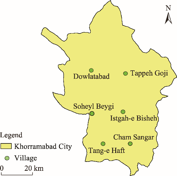
As the impact of climate change intensifies, climate migration (climate change-induced migration) has become a pressing global issue that requires effective adaptation strategies to lessen its effects. Therefore, this study delved into the complex relationship between climate change adaptation strategies and climate migration with food insecurity serving as a mediating factor. We collected sample data through face-to-face interviews in Khorramabad City, Iran from February to May in 2023. Using the Structural Equation Modeling (SEM), we explored how food insecurity influences the relationship between climate change adaptation strategies and climate migration. The findings showed that while climate change adaptation strategies can boost community resilience, their success is closely tied to levels of food insecurity. About 78.72% of the surveyed households experienced certain levels of food insecurity, increasing the risk of displacement due to climate-related disasters. Climate change adaptation strategies including economic strategies, irrigation management strategies, organic-oriented strategies, sustainable development-oriented strategies, and crop variety management strategies played a significant role in reducing climate migration. Moreover, we found that climate change adaptation strategies not only impact food security, but also shape migration decisions. This research underscores the importance of an integrated approach that links climate change adaptation strategies, climate migration, and food insecurity. This study emphasizes the importance of food security for formulating sustainable adaptation strategies.
Mohammad Reza PAKRAVAN-CHARVADEH , Jeyran CHAMCHAM , Rahim MALEKNIA . How climate change adaptation strategies and climate migration interact to control food insecurity?[J]. Regional Sustainability, 2025 , 6(3) : 100229 . DOI: 10.1016/j.regsus.2025.100229
Fig. 1. Overview of the study area. |
Table 1 Descriptive results of the Household Food Insecurity Access Scale (HFIAS). |
| Category | Question | Never (%) | Rarely (%) | Sometime (%) | Often (%) |
|---|---|---|---|---|---|
| Worrying about food availability | Q1: worrying about food availability | 38.21 | 30.11 | 17.19 | 14.49 |
| Preferred food | Q2: unable to eat preferred food | 41.62 | 29.41 | 21.57 | 7.40 |
| Limited variety of food | Q3: eating a limited variety of food | 43.21 | 26.02 | 20.28 | 10.49 |
| Unwanted food | Q4: eating foods that you have to eat unappealing food | 42.93 | 26.01 | 24.00 | 7.06 |
| Smaller meals | Q5: eating a smaller meal | 45.93 | 27.02 | 19.87 | 7.18 |
| Fewer meals | Q6: eating fewer meals in a day | 57.48 | 20.88 | 16.92 | 4.72 |
| Food shortage | Q7: no food to eat at home | 65.21 | 18.58 | 11.51 | 4.70 |
| Hunger at bedtime | Q8: going to bed hungry at night | 70.33 | 16.51 | 9.06 | 4.10 |
| Whole-day without any food | Q9: not eating for a whole day and night | 68.57 | 15.18 | 10.13 | 6.12 |
Table 2 Descriptive statistics of climate migration, food insecurity, and climate change adaptation strategies. |
| Factor | Item | Factor loading | Descriptive statistic | VIF | |||||||
|---|---|---|---|---|---|---|---|---|---|---|---|
| Original sample | Sample mean | SD | t-statistics | P-value | Mean | Average | CV | ||||
| Climate migration | I am willing to move to another region | 0.867 | 0.868 | 0.027 | 32.148 | 0.001 | 1.661 | 1.738 | 0.016 | 2.282 | |
| I feel prepared to migrate if necessary | 0.872 | 0.868 | 0.031 | 28.000 | 0.001 | 1.731 | 0.018 | 2.254 | |||
| I would be willing to leave my community | 0.937 | 0.937 | 0.009 | 104.111 | 0.001 | 1.823 | 0.005 | 3.326 | |||
| Food insecurity | Worrying about food availability | 0.588 | 0.590 | 0.087 | 6.782 | 0.001 | 1.194 | 0.804 | 0.073 | 1.337 | |
| Preferred food | 0.832 | 0.825 | 0.027 | 30.556 | 0.001 | 0.961 | 0.023 | 2.371 | |||
| Limited variety of food | 0.811 | 0.807 | 0.030 | 26.900 | 0.001 | 0.990 | 0.030 | 2.650 | |||
| Unwanted food | 0.846 | 0.841 | 0.028 | 30.036 | 0.001 | 0.951 | 0.029 | 3.504 | |||
| Smaller meals | 0.830 | 0.826 | 0.026 | 31.769 | 0.001 | 0.884 | 0.029 | 3.321 | |||
| Fewer meals | 0.764 | 0.764 | 0.033 | 23.152 | 0.001 | 0.693 | 0.048 | 2.215 | |||
| Food shortage | 0.701 | 0.704 | 0.052 | 13.538 | 0.001 | 0.561 | 0.093 | 2.387 | |||
| Going to bed hungry | 0.643 | 0.645 | 0.061 | 10.574 | 0.001 | 0.470 | 0.130 | 2.645 | |||
| Full day without eating | 0.462 | 0.465 | 0.078 | 5.962 | 0.001 | 0.540 | 0.144 | 1.724 | |||
| Climate change adaptation strategies | Economic strategies | Non-agricultural activity outside the farm | 0.946 | 0.929 | 0.133 | 6.985 | 0.001 | 1.772 | 1.763 | 0.075 | 3.586 |
| Non-agricultural employment (labor, sales, etc.) | 0.916 | 0.902 | 0.118 | 7.644 | 0.001 | 1.852 | 0.064 | 3.771 | |||
| Getting a loan | 0.915 | 0.899 | 0.123 | 7.309 | 0.001 | 1.871 | 0.066 | 3.323 | |||
| Using personal savings | 0.917 | 0.902 | 0.119 | 7.580 | 0.001 | 1.724 | 0.069 | 3.130 | |||
| Reducing household expenses | 0.944 | 0.924 | 0.143 | 6.462 | 0.001 | 1.671 | 0.086 | 3.681 | |||
| Livestock sale | 0.850 | 0.831 | 0.127 | 6.543 | 0.001 | 1.692 | 0.075 | 2.823 | |||
| Irrigation management strategies | Changing the irrigation system | 0.814 | 0.812 | 0.030 | 27.067 | 0.001 | 1.750 | 1.705 | 0.017 | 1.742 | |
| Improving the coverage of water transmission channels | 0.787 | 0.781 | 0.034 | 22.971 | 0.001 | 1.700 | 0.020 | 1.692 | |||
| Use of alternative water sources (rainwater, sewage, etc.) | 0.538 | 0.532 | 0.076 | 7.000 | 0.001 | 1.651 | 0.046 | 1.200 | |||
| Management of irrigation intervals | 0.712 | 0.712 | 0.052 | 13.692 | 0.001 | 1.832 | 0.028 | 1.414 | |||
| Watershed management activities (dam, gabion, trust, etc.) | 0.513 | 0.512 | 0.074 | 6.919 | 0.001 | 1.594 | 0.046 | 1.151 | |||
| Organic-oriented strategies | Weed management | 0.745 | 0.740 | 0.047 | 15.745 | 0.001 | 2.131 | 1.778 | 0.022 | 1.565 | |
| Use of organic fertilizer | 0.774 | 0.772 | 0.036 | 21.444 | 0.001 | 1.630 | 0.022 | 1.556 | |||
| Organic farming | 0.794 | 0.794 | 0.026 | 30.538 | 0.001 | 1.640 | 0.016 | 1.632 | |||
| Diversifying crops | 0.864 | 0.863 | 0.024 | 35.958 | 0.001 | 1.711 | 0.014 | 2.283 | |||
| Sustainable development -oriented strategies | Changing the crop cultivation deadline | 0.719 | 0.716 | 0.046 | 15.565 | 0.001 | 1.583 | 1.597 | 0.029 | 1.592 | |
| Conservation tillage | 0.729 | 0.724 | 0.044 | 16.455 | 0.001 | 1.684 | 0.026 | 1.780 | |||
| Agricultural land leveling | 0.739 | 0.734 | 0.047 | 15.617 | 0.001 | 1.910 | 0.025 | 1.777 | |||
| Changing the time of crop harvest | 0.546 | 0.540 | 0.063 | 8.571 | 0.001 | 1.590 | 0.040 | 1.301 | |||
| Multi-cropping | 0.813 | 0.811 | 0.025 | 32.440 | 0.001 | 1.570 | 0.016 | 2.012 | |||
| Compliance with crop rotation | 0.747 | 0.743 | 0.042 | 17.690 | 0.001 | 1.114 | 0.038 | 1.701 | |||
| Reducing the distance between crop rows | 0.656 | 0.653 | 0.052 | 12.558 | 0.001 | 1.732 | 0.030 | 1.604 | |||
| Crop variety management strategies | High-yielding varieties | 0.682 | 0.686 | 0.045 | 15.244 | 0.001 | 1.651 | 1.624 | 0.027 | 1.235 | |
| Using cold-resistant and pest-resistant varieties | 0.809 | 0.806 | 0.033 | 24.424 | 0.001 | 1.692 | 0.020 | 1.757 | |||
| Using varieties resistant to drought | 0.778 | 0.772 | 0.040 | 19.300 | 0.001 | 1.612 | 0.025 | 1.702 | |||
| Using varieties resistant to salt | 0.819 | 0.816 | 0.026 | 31.385 | 0.001 | 1.544 | 0.017 | 1.721 | |||
Note: SD, standard deviation; CV, coefficient of variation; VIF, Variance Inflation Factor. |
Table 3 Fitting results of the saturated and estimated models. |
| Criterion | Saturated model | Estimated model |
|---|---|---|
| SRMR | 0.068 | 0.068 |
| Squared Euclidean distance | 3.427 | 3.427 |
| Geodesic Distance | 1.082 | 1.082 |
| Chi-Square | 1749.170 | 1749.170 |
| NFI | 0.961 | 0.961 |
| RMS | - | 0.122 |
Note: -, no value. SRMR, Standardized Root Mean Square Residual; NFI, Normed Fit Index; RMS, Root Mean Square. |
Table 4 Reliability and validity of climate migration, food insecurity, and climate change adaptation strategies. |
| Factor | Cronbach’s Alpha | Dillon-Goldstein’s Rho | CR | AVE | |
|---|---|---|---|---|---|
| Climate migration | 0.872 | 0.880 | 0.922 | 0.797 | |
| Food insecurity | 0.882 | 0.940 | 0.904 | 0.522 | |
| Climate change adaptation strategies | Economic strategies | 0.961 | 1.002 | 0.969 | 0.837 |
| Irrigation management strategies | 0.706 | 0.742 | 0.810 | 0.568 | |
| Organic-oriented strategies | 0.805 | 0.807 | 0.873 | 0.633 | |
| Sustainable development-oriented strategies | 0.834 | 0.846 | 0.876 | 0.506 | |
| Crop variety management strategies | 0.775 | 0.779 | 0.856 | 0.599 | |
Note: CR, Composite Reliability; AVE, Average Variance Extracted. |
Table 5 Results of the Structural Equation Modeling (SEM). |
| Factor | Effect pathway | Original sample | Sample mean | SD | t-statistic | P-value | |
|---|---|---|---|---|---|---|---|
| Economic strategies | Climate migration | Direct effect | -0.046 | -0.048 | 0.009 | 4.721 | 0.000 |
| Indirect effect | -0.008 | -0.008 | 0.001 | 4.709 | 0.000 | ||
| Total effect | -0.054 | -0.040 | 0.008 | 4.580 | 0.000 | ||
| Food insecurity | Direct effect | -0.060 | -0.064 | 0.012 | 4.818 | 0.000 | |
| Irrigation management strategies | Climate migration | Direct effect | -0.201 | -0.209 | 0.079 | 2.542 | 0.011 |
| Indirect effect | -0.026 | -0.027 | 0.007 | 3.515 | 0.000 | ||
| Total effect | -0.227 | -0.236 | 0.082 | 2.770 | 0.006 | ||
| Food insecurity | Direct effect | -0.192 | -0.200 | 0.084 | 2.277 | 0.023 | |
| Organic-oriented strategies | Climate migration | Direct effect | -0.051 | -0.045 | 0.013 | 3.790 | 0.000 |
| Indirect effect | -0.024 | -0.024 | 0.006 | 3.559 | 0.000 | ||
| Total effect | -0.075 | -0.073 | 0.022 | 3.225 | 0.000 | ||
| Food insecurity | Direct effect | -0.177 | -0.179 | 0.049 | 3.554 | 0.000 | |
| Sustainable development-oriented strategies | Climate migration | Direct effect | -0.061 | -0.069 | 0.015 | 3.946 | 0.000 |
| Indirect effect | -0.004 | -0.004 | 0.012 | 0.345 | 0.731 | ||
| Total effect | -0.057 | 0.064 | 0.066 | 0.862 | 0.389 | ||
| Food insecurity | Direct effect | -0.031 | -0.032 | 0.009 | 3.396 | 0.000 | |
| Varity management strategies | Climate migration | Direct effect | -0.287 | -0.276 | 0.068 | 4.241 | 0.000 |
| Indirect effect | -0.008 | -0.009 | 0.012 | 0.668 | 0.505 | ||
| Total effect | -0.295 | 0.267 | 0.070 | 3.948 | 0.000 | ||
| Food insecurity | Direct effect | -0.062 | -0.064 | 0.085 | 0.725 | 0.469 | |
| Food insecurity | Climate migration | Direct effect | 0.134 | 0.131 | 0.059 | 2.282 | 0.023 |
Table S1 The description of all statistics for assessing the reliability and validity of the Structural Equation Modeling (SEM). |
| Statistic | Description | Equation | Explanation |
|---|---|---|---|
| λ | It describes the correlation between an observed variable and underlying latent variable. | $\lambda =\frac{\text{Cov}(X,Y)}{\sqrt{\text{Var}(X)\times \text{Var}(Y)}}$ | λ is the factor loading (Pearson correlation coefficient); Cov(X, Y) is the covariance between observed variable (X) and latent variable (Y); Var(X) is the variance of X; and Var(Y) is the variance of Y. The range of λ is between -1.000 and 1.000. λ value above 0.500 is considered acceptable relationship; λ value ranging from 0.400 to 0.500 is generally considered to reflect moderate relationship; while λ value below 0.400 may indicate weak relationship. |
| SRMR | It is calculated by the square root of the difference between the observed and predicted covariance matrices. | $\text{SRMR}=\sqrt{\frac{\sum\nolimits_{i=1}^{n}{{{({{O}_{ii}}-{{P}_{ii}})}^{2}}}}{n}}$ | SRMR is the Standardized Root Mean Square Residual; i is the observation value; n is the total number of observations; Oii is the observed covariance matrix; and Pii is the predicted covariance matrix. The range of SRMR is between 0.000 and 1.000, and SRMR value less than 0.080 is generally considered a good fitting. |
| dULS | It is the sum of squared differences between the observed and predicted covariance matrices. | ${{\text{d}}_{\text{ULS}}}=\sum\limits_{i=1}^{n}{\sum\limits_{j=1}^{m}{{{({{O}_{ij}}-{{P}_{ij}})}^{2}}}}$ | dULS is the Squared Euclidean distance; m is the total number of variables; Oij is the observed matrix for the observation ith and variable jth; and Pij is the predicted matrix for the observation ith and variable jth. There is no fixed range for dULS, but lower value indicates a better fitting. |
| dG | It is similar to dULS, but it takes into account the degrees of freedom. | ${{\text{d}}_{\text{G}}}=\sum\limits_{i=1}^{n}{\sum\limits_{j=1}^{m}{\frac{{{({{O}_{ij}}-{{P}_{ij}})}^{2}}}{\delta _{ij}^{2}}}}$ | dG is the Geodesic Distance; and δ2 ij is the variance associated with the observed matrix Oij. Like dULS, lower values indicate a better fitting, with no specific upper limit. |
| χ² | It is a statistical test used to determine if there is a significant association between categorical variables. | ${{\chi }^{2}}=\sum\limits_{l=1}^{L}{\frac{{{({{O}_{l}}-{{E}_{l}})}^{2}}}{{{E}_{l}}}}$ | χ² is the Chi-Square; L is the total number of categories; Ol is the observed frequency (count) for the lth category; and El is the expected frequency (count) for the lth category. The range of χ² is between 0.000 to infinity. Compared with the critical value based on the degrees of freedom, a lower value indicates a better fitting. |
| NFI | It compares the fitting of a proposed model to a baseline model, which usually represents a model of independence (i.e., no relationship between the variables). | $\text{NFI}=\frac{\chi _{\text{null}}^{2}-\chi _{\bmod \text{el}}^{2}}{\chi _{\text{null}}^{2}}$ | NFI is the Normed Fit Index; χ2 nul is the Chi-Square for the null model; and χ2 model is the Chi-Square for the specified model. The range of NFI is from 0.000 to 1.000. NFI value above 0.900 is typically considered indicative of a good fitting. |
| VIF | It quantifies how much the variance of an estimated regression coefficient increases when predictors are correlated. Moreover, it assesses multicollinearity in regression analysis. | $\text{VIF}=\frac{1}{1-R_{j}^{2}}$ | VIF is the Variance Inflation Factor; and R2 j is the coefficient of determination obtained by regressing the jth independent variable against all other variables. VIF=1.000 means no correlation; 5.000<VIF<10.000 means moderate correlation; 1.000≤VIF≤5.000 means high correlation; and VIF>10.000 means very high correlation. |
| CV | It measures the relative variability of a dataset compared to its mean. | $\text{CV}=\frac{\sigma }{\mu }$ | CV is the coefficient of variation; σ is the standard deviation (SD); and μ is the mean of the dataset. A higher CV indicates greater variability relative to the mean. |
| RMS | It measures the average of the squared differences (residuals) between the observed and predicted covariance matrices. | $\text{RMS}=\sqrt{\frac{1}{n}\sum\limits_{i=1}^{n}{{{({{O}_{i}}-{{P}_{i}})}^{2}}}}$ | Where RMS is the Root Mean Square; Oi is the observed value for the ith observation; and Pi is the predicted value for the ith observation. A value of RMS closer to 0.000 suggests that the model adequately captures the relationships in the data. |
| α | It measures the internal consistency and assesses how closely related a set of items are as a group. | $\alpha =\frac{k}{k-1}(1-\frac{\sum\nolimits_{g=1}^{k}{\delta _{{{Y}_{g}}}^{2}}}{\delta _{Y}^{2}})$ | α is the Cronbach’s Alpha; k is the number of items; δ2 Yg is the variance of the gth item; and δ2 Y is the variance of the total score. The range of α is between 0.000 and 1.000, with values above 0.700 generally being considered acceptable. |
| ρA | It is another measure of internal consistency and is often preferred over Cronbach’s Alpha, because it does not assume equal item loadings. | ${{\rho }_{A}}=\frac{\sum{\lambda _{g}^{2}}}{\sum{{{\lambda }_{g}}^{2}}+\sum{\lambda \sigma _{{{\varepsilon }_{g}}}^{2}}}$ | ρA is the Dillon-Goldstein’s Rho; λg is the factor loading of item; and $\sigma _{{{\varepsilon }_{g}}}^{2}$ is the error variance of item. Similar to Cronbach’s Alpha, values of ρA above 0.700 are considered acceptable. |
| CR | It reflects the factors’ reliability based on the factor loadings and error variances. | $\text{CR}=\frac{{{\left( \sum{{{\lambda }_{g}}} \right)}^{2}}}{{{\left( \sum{{{\lambda }_{g}}} \right)}^{2}}+\sum{\sigma _{{{\varepsilon }_{g}}}^{2}}}$ | CR is the Composite Reliability. CR value above 0.700 is considered acceptable. |
| AVE | It indicates how much of the variance in the observed variables (factors) is accounted for by the latent variables. | $\text{AVE}=\frac{\sum\nolimits_{g=1}^{k}{\lambda _{g}^{2}}}{k}$ | AVE is the Average Variance Extracted. AVE≥0.500 indicates good convergent validity and AVE<0.500 indicates concerns about the factor’s validity. |
Table S2 Discriminant validity results of the Fornell-Larcker criterion. |
| Factor | Climate migration | Economic strategies | Food insecurity | Irrigation management strategies | Organic- oriented strategies | Sustainable development- oriented strategies | Crop variety management strategies |
|---|---|---|---|---|---|---|---|
| Climate migration | 0.893 | ||||||
| Economic strategies | -0.090 | 0.915 | |||||
| Food insecurity | 0.237 | -0.119 | 0.722 | ||||
| Irrigation management strategies | -0.465 | 0.248 | -0.238 | 0.753 | |||
| Organic-oriented strategies | -0.330 | 0.180 | -0.244 | 0.503 | 0.795 | ||
| Sustainable development -oriented strategies | 0.316 | -0.429 | 0.144 | -0.560 | -0.386 | 0.711 | |
| Crop variety management strategies | 0.478 | -0.122 | 0.136 | -0.643 | -0.457 | 0.432 | 0.774 |
Table S3 Discriminant validity results of the Heterotrait-Monotrait Ratio (HTMT). |
| Factor | Climate migration | Economic strategies | Food insecurity | Irrigation management strategies | Organic- oriented strategies | Sustainable development- oriented strategies | Crop variety management strategies |
|---|---|---|---|---|---|---|---|
| Economic strategies | 0.095 | ||||||
| Food insecurity | 0.251 | 0.117 | |||||
| Irrigation management strategies | 0.581 | 0.278 | 0.274 | ||||
| Organic-oriented strategies | 0.392 | 0.201 | 0.261 | 0.671 | |||
| Sustainable-oriented strategies | 0.368 | 0.465 | 0.161 | 0.704 | 0.472 | ||
| Crop management strategies | 0.572 | 0.146 | 0.143 | 0.844 | 0.565 | 0.524 |
| [1] |
|
| [2] |
|
| [3] |
|
| [4] |
|
| [5] |
|
| [6] |
|
| [7] |
|
| [8] |
|
| [9] |
|
| [10] |
|
| [11] |
|
| [12] |
|
| [13] |
|
| [14] |
|
| [15] |
|
| [16] |
|
| [17] |
|
| [18] |
|
| [19] |
|
| [20] |
|
| [21] |
|
| [22] |
|
| [23] |
|
| [24] |
|
| [25] |
|
| [26] |
|
| [27] |
|
| [28] |
|
| [29] |
|
| [30] |
|
| [31] |
|
| [32] |
|
| [33] |
|
| [34] |
|
| [35] |
|
| [36] |
|
| [37] |
|
| [38] |
|
| [39] |
|
| [40] |
|
| [41] |
|
| [42] |
|
| [43] |
|
| [44] |
|
| [45] |
|
| [46] |
|
| [47] |
|
| [48] |
|
| [49] |
|
| [50] |
|
| [51] |
|
| [52] |
|
| [53] |
|
| [54] |
|
| [55] |
|
| [56] |
|
| [57] |
|
| [58] |
|
| [59] |
|
| [60] |
|
| [61] |
|
| [62] |
|
| [63] |
|
| [64] |
|
| [65] |
|
| [66] |
|
/
| 〈 |
|
〉 |