Full Length Article

Application of Cellular Automata and Markov Chain model for urban green infrastructure in Kuala Lumpur, Malaysia

  • Jafarpour Ghalehteimouri KAMRAN , * ,
  • Che Ros FAIZAH ,
  • Rambat SHUIB
Expand
  • Disaster Preparedness & Prevention Centre, Malaysia - Japan International Institute of Technology, Universiti Teknologi Malaysia, Kuala Lumpur, 54100, Malaysia
*E-mail address: (Jafarpour Ghalehteimouri KAMRAN).

Received date: 2024-02-25

  Revised date: 2024-09-03

  Accepted date: 2024-11-16

  Online published: 2025-08-13

Abstract

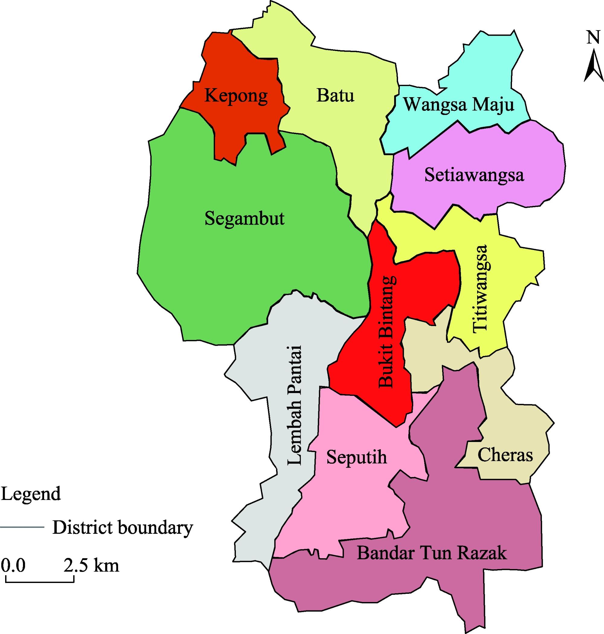
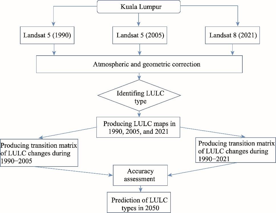
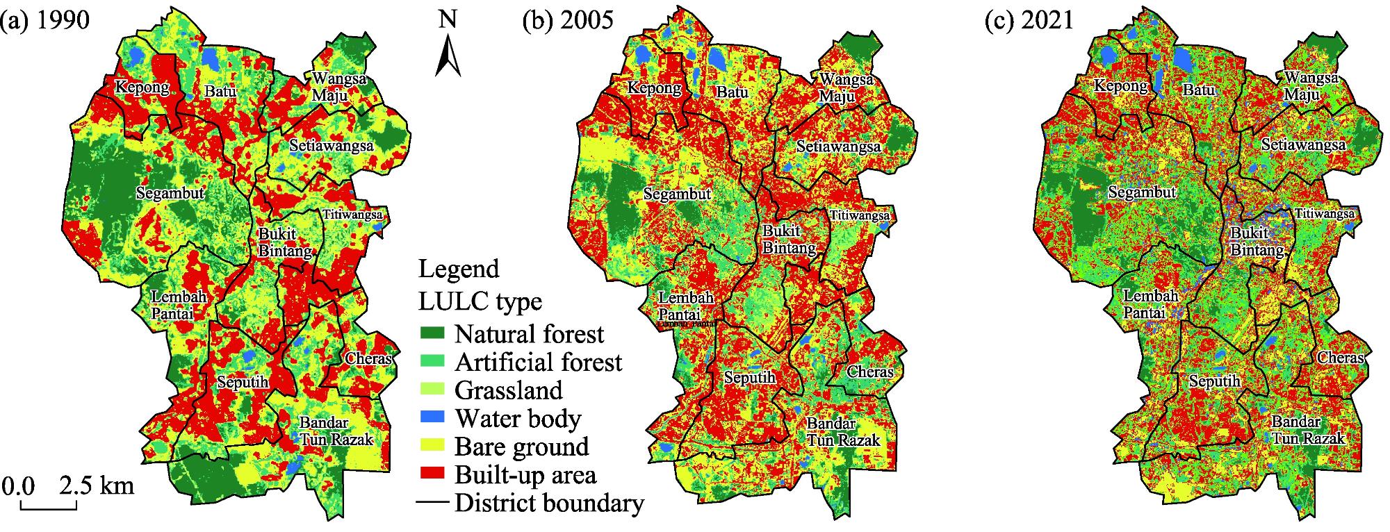
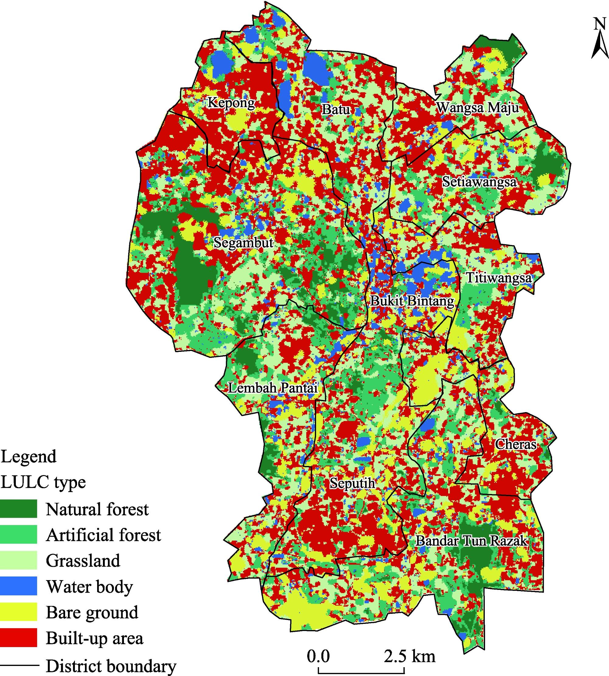
Kuala Lumpur of Malaysia, as a tropical city, has experienced a notable decline in its critical urban green infrastructure (UGI) due to rapid urbanization and haphazard development. The decrease of UGI, especially natural forest and artificial forest, may reduce the diversity of ecosystem services and the ability of Kuala Lumpur to build resilience in the future. This study analyzed land use and land cover (LULC) and UGI changes in Kuala Lumpur based on Landsat satellite images in 1990, 2005, and 2021and employed the overall accuracy and Kappa coefficient to assess classification accuracy. LULC was categorized into six main types: natural forest, artificial forest, grassland, water body, bare ground, and built-up area. Satellite images in 1990, 2005, and 2021 showed the remarkable overall accuracy values of 91.06%, 96.67%, and 98.28%, respectively, along with the significant Kappa coefficient values of 0.8997, 0.9626, and 0.9512, respectively. Then, this study utilized Cellular Automata and Markov Chain model to analyze the transition of different LULC types during 1990-2005 and 1990-2021 and predict LULC types in 2050. The results showed that natural forest decreased from 15.22% to 8.20% and artificial forest reduced from 18.51% to 15.16% during 1990-2021. Reductions in natural forest and artificial forest led to alterations in urban surface water dynamics, increasing the risk of urban floods. However, grassland showed a significant increase from 7.80% to 24.30% during 1990-2021. Meanwhile, bare ground increased from 27.16% to 31.56% and built-up area increased from 30.45% to 39.90% during 1990-2005. In 2021, built-up area decreased to 35.10% and bare ground decreased to 13.08%, indicating a consistent dominance of built-up area in the central parts of Kuala Lumpur. This study highlights the importance of integrating past, current, and future LULC changes to improve urban ecosystem services in the city.

Cite this article

Jafarpour Ghalehteimouri KAMRAN , Che Ros FAIZAH , Rambat SHUIB . Application of Cellular Automata and Markov Chain model for urban green infrastructure in Kuala Lumpur, Malaysia[J]. Regional Sustainability, 2024 , 5(4) : 100179 . DOI: 10.1016/j.regsus.2024.100179

1. Introduction

The rapid changes in land use and land cover (LULC) are leading to environmental hazards and climate change, such as soil erosion, air pollution, and heat islands, as well as socioeconomic problems and uneven spatial development. Despite cities covering only 2.00% of the world’s land, they are major contributors to greenhouse gas emissions, accounting for 70.00%-80.00% of the total greenhouse gas emissions (Masi et al., 2018; Schwab, 2021). The rapid urbanization and LULC changes have reduced Urban Green Infrastructure (UGI) and impacted the delivery of ecosystem services (Kajosaari et al., 2024). Urban ecosystem services have been studied by biogeographers for a long time, predating the Millennium Ecosystem Assessment (2005), as shown in earlier studies (Monte, 1978; Seutin et al., 1994; van Veller et al., 2000). Despite their significance, the successful utilization of urban ecosystem services in research is often overlooked. Various factors have contributed to the disconnect between urban ecosystem services and UGI. The complexity of urban ecosystems poses challenges in understanding and incorporating their diverse components (Tzoulas et al., 2007; Kuenzer, 2011). Moreover, urban development typically involves multiple stakeholders, complicating the coordination and integration of their needs and interests. Insufficient funding and resources for urban ecosystem services and UGI development can result in fragmented projects and hinder integration efforts (Keeley et al., 2013; Estrada-Carmona et al., 2014). The decline of essential ecosystem services is a result of urbanization, population growth, and increased built-up area. The impact of urbanization and LULC changes on urban ecosystem services is significant. Research on ecosystem services, including sustainable food production and conservation efforts, is growing in importance in environmental protection. However, the uncontrolled consumption of natural resources only increases the demand for these valuable ecosystem services (Jordan et al., 2010). A decline in urban ecosystem services can be attributed to the impact of natural hazards or human modification of the environment. One of the most significant human impacts on urban ecosystem services is LULC changes. Depending on the value of changes, there can be significant changes in the quality of the ecosystem services previously provided.
Urban ecosystem services are highly vulnerable to the rapid and inconsistent changes in urban LULC, referred to as urban ecosystem service disturbances (Chaudhary et al., 2015). These quick decisions not only disrupt the proper utilization of urban ecosystem services, but also jeopardize the current and future urban environmental objectives (Clerici et al., 2019; Chen et al., 2024). The degradation of urban ecosystem services undermines urban sustainable development goals due to swift changes in LULC, which are widely acknowledged as the primary driving factor of urban environmental deterioration. Urban ecosystem services, particularly UGI, play a vital role in human well-being, especially in terms of nutrition and health. Urban ecosystem services are categorized into provisioning, regulating, cultural, and supporting functions (Millennium Ecosystem Assessment, 2005). While these functions are interconnected, supporting function is crucial for other three functions. Additionally, variations in urban ecosystem services can be observed not only within neighboring cities but also across countries. Factors such as soil type, temperature, green spaces, agricultural lands, and rainfall patterns are considered in LULC planning (Kopperoinen et al., 2022). UGI is a key provider of urban ecosystem services, aiding in the reduction of greenhouse gas emissions, prevention of soil erosion, mitigation of flooding, improvement of air quality, and enhancement of the cultural and aesthetic aspects of urban landscapes. Therefore, an effective evaluation of urban ecosystem service should be capable of tracking and analyzing trends from the past to the present. Subsequently, historical and current data should be utilized to analyze potential problems arising from changes in UGI.
Ecosystem services play a crucial role in improving the environmental quality and the resilience of an area by identifying the main factors and disturbances that affect their quality (Mitchell et al., 2021). The impacts of LULC changes on UGI is essential to understanding current and future patterns in UGI (Dong et al., 2015). Recognizing urban ecosystem services and their contributions has long been important (Lamarque et al., 2011). The rapid LULC changes in urban areas have potential implications that require reliable and precise assessment (Desta and Fetene, 2020). Remote sensing and spatial analytic tools are widely used in geographic studies (Chen et al., 2018) and can effectively assess LULC changes (Congalton, 1991; Kattenborn et al., 2021; Piralilou et al., 2022). High-resolution and long time series satellite data are crucial for accurate assessment of LULC changes and informing land development strategies (Jalayer et al., 2023). Understanding LULC changes and identifying beneficial urban ecosystem services can help mitigate future adverse effects (Uddin et al., 2015). Proactive assessments of LULC changes using satellite data can inform future conservation plans and be integrated into current planning and actions (Gambo et al., 2018). Advanced monitoring and computation technologies, along with methods for interpreting satellite data results, enhance the quality and accuracy of assessments. Various methods, such as Cellular Automata and Markov Chain model, are used for LULC predictions, focusing on spatiotemporal dynamics and big data analysis (Ghalehteimouri et al., 2022).
Understanding and assessing UGI is essential in tropical cities because of the critical urban ecosystem services they provide, which help maintain ecological balance, support human well-being, and mitigate the impacts of climate change. UGI plays a significant role in improving the environmental quality, aesthetics, and the overall livability of cities in Southeast Asia. Previous studies in Malaysia (Tan et al., 2010; Hua, 2017; Ghalehteimouri et al., 2024), Indonesia (Agaton et al., 2016; Maheng et al., 2021), and Thailand (Ongsomwang et al., 2019) have offered valuable insights into UGI, urban ecosystem services, and LULC changes. Abdullah and Nakagoshi (2007) conducted a study focusing on the reduction of green infrastructure at the state level. Monitoring changes in UGI is crucial for understanding how urban ecosystem services like carbon sequestration and water management contribute to climate change and inform future climate change adaptation and mitigation strategies. Urban ecosystem services can help address challenges related to urbanization and enhance risk reduction strategies that have been neglected by the public and government for a long time. Despite facing significant challenges, integrating ecosystem services into urban studies is essential for a comprehensive understanding of urban environments. The use of Cellular Automata and Markov Chain model in this study facilitates the integration of various aspects of urban ecosystem services into urban planning and policymaking.
This study utilized accurate and comprehensive data of LULC and highlighted previously overlooked LULC changes in tropical cities with less emphasis on prediction. Unlike previous study that primarily focused on climatic conditions (Esmaeili et al., 2023), this study introduced a new classification that considered land exposure and analyzed the changes of UGI. Remote sensing and spatial analytic tools play a crucial role in analyzing the change trends of different LULC types. Six distinct LULC types were identified, with a specific focus on UGI including natural forest, artificial forest, and grassland, as well as non-UGI covering water body, bare ground, and built-up area. The study of UGI in Kuala Lumpur (Malaysia) has significant implications for assessing urban ecosystem services and improving current and future urban resilience. The urbanization of Kuala Lumpur is influenced by the growth of urban population, making the urban ecosystem essential in determining the city’s resilience level.

2. Materials and methods

2.1. Study area

Kuala Lumpur is the capital and largest city in Malaysia (Fig. 1). It has a population of 2.08×10⁶ in 2024 and covers an area of 243.00 km2, making it as Malaysia’s largest metropolis. The influence of city extends to the surroundings of Klang Valley, with a total population of 7.63×10⁶ in 2018. Greater Kuala Lumpur, also known as the Klang Valley, is an urban agglomeration with the population of 8.80×10⁶ in 2024 (Dewan Bandaraya Kuala Lumpur, 2022; Malaysia Tourism Promotion Board, 2022; Federal Territory of Kuala Lumpur, 2024).
Fig. 1. Overview of the study area.

2.2. Data source

This study emphasized the significance of rapid urbanization in influencing urban ecosystem services through the analysis of long-term Landsat data from Landsat 5 in 1990 and 2005, and Landsat 8 in 2021. We specifically identified six LULC types including natural forest, artificial forest, grassland, water body, bare ground, and built-up area (Table 1).
Table 1 Identified land use and land cover (LULC) types of Kuala Lumpur.
No. Type Description
1 Natural forest The original forests remained in Kuala Lumpur.
2 Artificial forest Trees that planted by human around buildings and houses.
3 Grassland Football fields, parks, and empty lands with growing grasses.
4 Water body Ponds, swamps, lakes, rivers, ditches, and lagoons.
5 Bare ground Any open exposed lands without vegetation cover.
6 Built-up area Residential areas, factories, apartments, roads, and constructions.
The main objective of this study was to assess the spatial expansion of UGI in Kuala Lumpur by classifying LULC types using satellite images, literature, and field observations. Maps were created using the Maximum Likelihood Classifier in 1990, 2005, and 2021 to analyze the spatial distribution and changes of LULC with a particular focus on UGI in Kuala Lumpur.

2.3. Data analysis

This study used Cellular Automata and Markov Chain model to analyze the quality, spatial expansion, transformation, and distribution of each identified LULC type as well as their interactions.. The calculation steps of this method are as follows:
(1) Preprocessing. Radiometric and atmospheric corrections were used to facilitate the differentiation of LULC types.
(2) Creating red, green, and blue bands. Typically, LULC data collection relies on natural band data, which varies between different satellites and is known as red, green, and blue bands. Data from Landsat 5 were combined by blue,
green, and red bands, and data from Landsat 8 were combined by red, green, and blue bands. This natural color composite uses a band combination of red, green, and blue, closely resembling what human can see. Healthy vegetation appears green, while unhealthy vegetation presents brown. Without combining these bands, built-up area appears white and grey clolors, and water body shows dark blue or black clolor (Vali et al., 2020; Mountrakis and Heydari, 2023).
(3) Satellite classification. Using supervised or unsupervised classification methods to categorize pixels into different LULC types. Support Vector Machine (SVM) was applied for better data collection and monitoring. Finally, natural forest, artificial forest, grassland, water body, bare ground, and built-up area were selected for evaluation and prediction of LULC changes (Aziz et al., 2024).
(4) Accuracy assessment. The accuracy was obtained through the application of the Kappa coefficient (He, 2024). The Kappa coefficient serves as an indicator of agreement between two classifiers, accounting for the potential agreement that could happen by random chance. It delivers a normalized agreement measure, spanning from -1.0000 to 1.0000; it can be calculated as follows:
$T=\frac{(TS-TCS)-\sum (\text{Column total}\times \text{Row total})\text{ }}{T{{S}^{2}}\sum \text{Column total}\times \text{Row total}}$,
where T is the Kappa coefficient; TS is the total classification; and TCS is the total classification score.
We validated the classification results using field observation data obtain in 2021 and high-resolution imagery to ensure the accuracy of LULC types. The Kappa coefficient serves as an indicator of agreement. A Kappa coefficient value below zero signifies an agreement worse than chance, while a Kappa coefficient value of zero denotes an agreement at the level expected by chance. When the Kappa coefficient value falls between 0.0000 and 1.0000, it indicates agreement surpassing what would be anticipated by chance, with the higher values representing stronger an agreement. A Kappa coefficient value of 1.0000 signifies a state of perfect agreement. Moving on to the calculation of total accuracy, also referred to as the overall accuracy, it’s a rather straightforward process. This involves dividing the count of correctly classified changes comprising true positives and true negatives by the total number of changes, as illustrated in Equation 2:
$\text{OA}=\frac{Tc\text{ }}{Tr}\times 100%$,
where OA is the overall accuracy (%); Tc is the total number of correctly classified pixels; and Tr is the total number of referenced pixels.
(5) Change detection. This study used classified maps from different years to identify and quantify changes in LULC. Many change detection studies focus on anlyzing urbanization and UGI changes (Moharrami et al., 2024; Pham et al., 2024).
(6) Analysis and interpretation. We analyzed the patterns and driving factors of LULC changes, and interpreted the findings in the context of environmental, social, and economic conditions. These are identifiable through the socio-economic interactions among LULC changes, UGI, and general policy in the planning system (Wilmer et al., 2024).

2.4. Application of Cellular Automata and Markov Chain model

Two matrices were created using Cellular Automata and Markov Chain model to analyze the transition probabilities of different LULC types in Kuala Lumpur during 1990-2005 and 1990-2021 (Fig. 2). Cellular Automata and Markov Chain model aims to describe spatial interactions and cell memory in relation to neighbors. Each cell has an internal model, and values are shared throughout the system. When cells are updated, we will update neighboring cells based on the neighboring rules and general transformation. The memory mechanism in Cellular Automata and Markov Chain model considers previous changes to assess future spatiotemporal patterns of LULC changes (Alonso-Sanz and Martin, 2007). Cellular Automata and Markov Chain model is a grid-based dynamic model with strong spatial computing capabilities, working with discrete time, space, and states. Despite limitations in time causality and spatial connections, Cellular Automata and Markov Chain model can analyze the spatiotemporal development of complex systems (Lu et al., 2019).
Fig. 2. Workflow adopted in this study. LULC, land use and land cover.
According to Jordan et al. (2010), the improvement of population increases the demand for urban ecosystem services. Ecosystem valuation can be approached through both monetary and non-monetary ways. The projected global monetary value of environmental services was 1.25×10¹⁴ USD in 2014 (FAO, 2021). This amount increased according to the latest study (Morizet-Davis et al., 2023), which analyzed the global Gross Ecosystem Product (GEP) across 179 countries, revealing that ecosystems contributed 1.12×10¹⁴-1.97×10¹⁴ USD to the global economy in 2018. The ratio of GEP to GDP was obtained to be 1.85. Forest and wetland ecosystems were highlighted as the most important providers, making up almost 80.00% of the global GEP (Morizet-Davis et al., 2023). However, due to the dynamic nature of urban ecosystem systems, there is insufficient knowledge about the functions of ecosystem services, notably UGI. Changes in the vegetation index have the ability to affect both regional air circulation and long-term water table levels. As a result, spatiotemporal analysis is required to assess existing conditions and estimate future changes in UGI.

2.4.1. Cellular Automata process

This study used Cellular Automata to estimate the overall nature and behavior of system transitions by detecting frequent movements between cells and their neighbors, particularly when evaluating specific LULC types. Additionally, the exchange of various LULC types provides accurate insights into UGI changes. In Cellular Automata process, LULC type is represented by square cells in a limited area, with each cell containing an identical finite automaton. The surrounding cells include four additional cells, except for diagonal neighbors. A cell’s state at time t is determined by the states of its immediate neighborhood, the transition function of the finite automaton associated with each cell (denoted as f), and the state of the cell at time t+1. These associated finite automata within each cell encompass a distinct quiescent state denoted as v0, which serves as a reference state as shown in Equation 3. Except for a small number of cells, all cells are in a quiescent condition at any given time step. Each cell’s linked finite automaton has 29 distinct states. The following computation and built-up features are produced by a specific transition function f, which is described as follows:
f=(v0, v0, v0, …, v0)=v0.

2.4.2. Markov Chain process

The Markov Chain process works with a series of random variables. Therefore, it is preferable to first define the random variable, support, probability function, and conditional probability. This expression is written in mathematical notation as follows:
(Ω, F, P) X→(R, B, Px),
where Ω is the event space; F is the sigma algebra of events; P is the probability; X is the random variable; R is the set of real numbers; B is the Borel set, which is a collection of subsets of R that can be formed using countable unions, intersections, and complements of open intervals (essentially the sigma algebra on the real line); and Px is the probability distribution of the specific value x, which is shown to be a function of the event space and a set of subsets of real numbers. It means that the random variable (X) transforms the sample space members into real numbers, the event space members into the Borel set (B) of real numbers, and the event probability function into the probability of a random variable.
The support of a random variable is the set of values where it has a positive probability, typically denoted as the probability function for a random variable X. It calculates the probability for the support values of the random variable and considers it as zero for the rest of the real numbers. Essentially, for a discrete random variable, the probability function corresponds to the probability of a specific event (Niya et al., 2019; Biswas et al., 2020), as shown in Equation 5:
P(x)=P(X=x),
where P(x)=P(X=x) simply states that the probability function P(x) is equal to the probability that the random variable X equals the specific value x. The probability function represents the probability distribution for various values of the support of X.
The joint probability function P(x, y) is defined over the support of the random variables X and Y, meaning that it is only non-zero for specific values of x and y where both values are within the support of their respective variables. When it is necessary to calculate the probability of two events happening simultaneously, the joint probability function is utilized. Therefore, when X and Y are random variables, determining the probability of their events occurring for all support values is known as a joint probability function, as follows:
P(x, y)=P(X=x, Y=y).
Equation 6 explains the probability of X taking on a specific value x and Y taking on a specific value y. The conditional probability function is utilized to determine the likelihood of an event occurring when another event is known. For two independent discrete random variables X and Y, the conditional probability is calculated as follow (Campos et al., 2022):
$P(X=x|Y=y)=\frac{P(X=x,Y=y)\text{ }}{P(Y=y)}$.
The conditional probability will not be defined if the random variable P(Y=y)=0. For independent random variables, the conditional probability is given by P(X=x|Y=y)=P(X=x). Independence implies that the value of Y does not influence the probability of X, so the conditional probability P(X=x|Y=y) is the same as the marginal probability P(X=x). In terms of conditional probability function or joint probability function, if X and Y are independent, it is shown as follows:
P(X=x|Y=y)=P(X=x) or P(X=x|Y=y)=P(X=x)P(Y=y).
A sequence of random variables is also a collection of random variables indexed by natural numbers. For example, Xt denotes a random variable in time t. As a result, the sequence of the random variable is {Xt, t∈Q}, where Q is the index set representing time or location. The sequence or random process is called continuous if the collection t∈Q contains continuous values (Talagrand, 2005; Johnson and Willsky, 2013; Austin et al., 2021). If the specified value is Q and it is discrete, the process is classified as a discrete process.

2.4.3. Markov chain and discrete-time Markov process

A Markov Chain is defined as the possibility of changing the situation from time t to time t+1 independently of previous states (Yakir, 1994). This proposition is demonstrated as follows:
Pr(Xt+1=x|X1=x1, X2=x2, …, Xn=xt)=Pr(Xt+1=x|Xt=xt).
It is obvious that when calculating this conditional probability, Pr(X1=x1, X2=x2, …, Xn=xn)>0; otherwise, the conditional probability cannot be calculated. This possibility means that in the random process, the path (X1=x1, X2=x2, …, Xn=xn) has a positive probability. Therefore, in the Markov random process, the mentioned path can lead to the point Xt=xt.
As a result, a Markov random process is one that has the Markov property and is introduced as an infinite sequence of random variables. If the state space in this process is finite, the process is referred to as finite; if not, it is referred to as endless. The structure of a Markov random process is related to the characteristics of the Markov Chain. It should be mentioned that a directed graph is often used to depict the Markov Chain. Grebík et al. (2023) valued this graph’s edges according to how likely a vertex will transition to another.
The matrix of the Markov Chain can be shown as a “Transition Probability Matrix” since this graph can be represented as a matrix (Zadbagher et al., 2018). The probability of moving from the state i to j is displayed in this instance by writing the matrix elements as Pij. In this manner, the transfer matrix (P) for the aforementioned graph can be computed in the following sequence according to the vertex values (values associated with the set of state space). This is represented as:
$P=\left[ \begin{matrix} {{P}_{11}} & {{P}_{12}} & 0 \\ 0 & {{P}_{22}} & {{P}_{23}} \\ {{P}_{31}} & 0 & {{P}_{33}} \\\end{matrix} \right]$.
Additionally, in the Markov Chain, Pij typically denotes the probability of transitioning from state i to state j. This represents the likelihood that a system in state i will move to state j in the next step. The sum of all transition probabilities from state i to possible state j was calculated as follows:
$\sum\nolimits_{j=1}^{k}{{{P}_{ij}}=1}$.
The sum is calculated over all possible states (ranging from 1 to k) that the system can transition to. The equation equals to 1, which indicates that the total probability of transitioning from state i to possible state j must add up to 1. This principle of probability ensures that the system will transition to one of the possible states after a step in time, as illustrated in Equation 11.
It is important to mention that in a uniform Markov Chain process, the probability of transitioning from state i to state j in n steps is calculated by taking the states i and j of the transition probability matrix raised to the power of n. The calculation formulas are as follows:
$P_{ij}^{n}=\sum\nolimits_{r\in s}{P_{ij}^{k}}P_{rj}^{n-k}$,
${{P}_{r}}({{X}_{n=F}})=\sum\nolimits_{r\in s}{{{P}_{rj}}{{P}_{r}}({{X}_{n-1}}=r)=\sum{{{P}_{rj}}}}(n){{P}_{r}}({{X}_{0}}=r),$
where Pn ij denotes the probability of moving from state i to state j in exactly n steps within a Markov Chain; ΣrS is performed over all possible intermediate states r within the state space S; Pk ij represents the probability of transitioning from state i to an intermediate state j in k steps; Pn−k rj indicates the probability of transitioning from intermediate state r to final state j in the remaining nk steps; Pr(Xn=F) indicates the probability of the system being in state F at the nth move (time step); Prj means the probability of transitioning from state r to an intermediate state j; Pr(Xn-1=r) is the probability of the system being in state r at the (n−1)th step; and Pr(X0=r) is the initial distribution, indicating the probability of the system starting in state r at the beginning (step 0). The distribution’s general form for subsequent moves is represented with n as the subscript and not the exponent.

3. Results

3.1. Transition matrix of land use and land cover (LULC) during 1990-2005 and 1990-2021

We established the transition matrix of pixel changes and probability changes of different LULC types during 1990-2005 by Cellular Automata and Markov Chain model. From Table 2 we can see that grassland, bare ground, and built-up area had the significant growth.
Table 2 Transition matrix of pixel changes of different land use and land cover (LULC) types during 1990-2005.
Built-up area Bare ground Water body Grassland Artificial forest Natural forest
2427 6569 169 875 481 4435 Natural forest
10,364 15,739 1593 2372 9644 3019 Artificial forest
3273 4408 41 820 2026 490 Grassland
294 490 2451 84 618 116 Water body
41,206 30,282 364 3451 11,402 1718 Bare ground
66,886 28,679 47 1447 7440 325 Built-up area
Table 3 shows a notable decrease in natural forest during 1990-2005. Furthermore, the transition among grassland, bare ground, and built-up area was more common compared to other LULC types. Although water body was relatively small, there was a noticeable upward trend, suggesting that water body was likely to expand during this period.
Table 3 Transition matrix of probability changes of different LULC types during 1990-2005.
Built-up area Bare ground Water body Grassland Artificial forest Natural forest
0.1259 0.3406 0.0087 0.0454 0.2494 0.2299 Natural forest
0.2425 0.3683 0.0373 0.0555 0.2257 0.0706 Artificial forest
0.2960 0.3986 0.0037 0.0742 0.1832 0.0443 Grassland
0.0725 0.1210 0.6048 0.0207 0.1524 0.0286 Water body
0.4660 0.3425 0.0041 0.0390 0.1290 0.0194 Bare ground
0.6381 0.2736 0.0004 0.0138 0.0710 0.0031 Built-up area
We also established the transition matrix of pixel changes and probability changes of different LULC types during 1990-2021 by Cellular Automata and Markov Chain model. Table 4 shows a significant transition from natural forest and artificial forest to other LULC types. Decreases in natural forest and artificial forest and increases in bare ground and grassland occurred from 1990 to 2021, as shown in Table 5.
Table 4 Transition matrix of pixel changes of different LULC types during 1990-2021.
Built-up area Bare ground Water body Grassland Artificial forest Natural forest
3698 2562 500 3322 4131 8058 Natural forest
9621 4632 2468 10,071 10,301 3973 Artificial forest
15,481 7370 1691 19,225 18,687 3939 Grassland
775 778 7513 1019 965 309 Water body
13,189 5191 1237 10,694 4886 675 Bare ground
49,304 14246 2459 22,473 4803 129 Built-up area
Table 5 Transition matrix of probability changes of different LULC types during 1990-2021.
Built-up area Bare ground Water body Grassland Artificial forest Natural forest
0.1660 0.1150 0.0225 0.1492 0.1855 0.3618 Natural forest
0.2343 0.1128 0.0601 0.2452 0.2508 0.0968 Artificial forest
0.2332 0.1110 0.0255 0.2896 0.2815 0.0593 Grassland
0.0683 0.0685 0.6614 0.0897 0.0849 0.0272 Water body
0.3677 0.1447 0.0345 0.2981 0.1362 0.0188 Bare ground
0.5278 0.1525 0.0263 0.2406 0.0514 0.0014 Built-up area

3.2. Spatiotemporal changes of LULC during 1990-2021

In 1990, Kuala Lumpur was abundant in natural forest, creating a lush and green landscape (Fig. 3). However, natural forest was mostly concentrated in Bandar Tun Razak and Segambut districts. In contrast, districts like Wangsa Maju, Titiwangsa, and Lembah Pantai had scattered patches of natural forest. The central part of Kuala Lumpur, particularly Bukit Bintang District, was densely developed and lacked significant natural forest due to its role as a hub for commercial and administrative activities.
Fig. 3. Spatical distribution of LULC types of Kuala Lumpur in 1990 (a), 2005 (b), and 2021 (c).
In 1990, Kuala Lumpur’s UGI was in a favorable state. Natural forest covered 15.22% of the total area, artificial forest covered 18.51%, and grassland occupied 7.80% (Fig. 3a). Together, UGI accounted for a substantial 41.53% of the total area, with natural forest and artificial forest being the dominant LULC types. In contrast, the water body made up only 0.86% of the total area, while bare ground covered 27.16%, and built-up area occupied 30.45%. The expansion of UGI in 1990 was mainly concentrated in the western region of Kuala Lumpur, while the other parts of Kuala Lumpur had lower UGI, particularly in terms of natural forest.
In 2005, Kuala Lumpur showed significant changes in LULC compared to 1990, with a loss of over 60.00% for its natural forest and artificial forest (Fig. 3b). The LULC type of this city predominantly changed to built-up area, marking a substantial departure from its previous LULC types. Central districts like Bukit Bintang were fully developed, while Segambut and Bandar Tun Razak districts experienced significant losses in natural forest due to the rapid urbanization and land transformation.
After 2005, there were significant changes related to the implementation of the National Physical Plan. In 2005, there was a notable change in the distribution of LULC in Kuala Lumpur (Ghalehteimouri and Ros, 2020). Natural forest sharply declined to 6.99%. Artificial forest experienced a slower decline, reaching 15.80%, while grassland decreased to 4.29%. As a result, the total UGI experienced a significant drop, falling to 27.80%. On the other hand, water body increased to 1.46%, which doubled compared to 1990 but remained relatively low. Non-UGI was constituted by bare ground (31.56%) and built-up area (39.90%), which occupied a substantial portion, accounting for 71.46% of the total area. These changes signify a shift in LULC types of Kuala Lumpur, which is characterized by a decrease in UGI and an increase in non-UGI.
In 2021, Kuala Lumpur showed a slight increase in natural forest and artificial forest (Fig. 3c). However, this increase was not enough to be considered a wholly positive change in the overall status of UGI. The gradual urbanization toward natural forest in Segambut and Bandar Tun Razak districts has been eroding this valuable natural forest. The current small patches of natural forest and artificial forest in Segambut, Bandar Tun Razak, Wangsa Maju, and Titiwangsa districts have been preserved due to their higher elevations and the difficulties associated with utilizing these lands. However, recent trends indicated that these areas are undergoing changes, with new machinery and technologies, particularly in Segambut District.
In 2021, there has been a slight increase in natural forest, reaching 8.20% (Fig. 3c). Artificial forest has remained relatively stable at 15.16%, while grassland has experienced significant growth, reaching 24.30%. This notable increase in grassland has contributed to the overall value of UGI, which reached its highest value during 1990-2021. Water body has increased to 4.16%. In contrast, there was a significant decrease in non-UGI, with bare ground declining to 13.08% and built-up area decreasing to 35.10%.

3.3. Prediction of LULC in 2050

This study utilized time series data to accurately predict LULC types in Kuala Lumpur’s in 2050. The application of Cellular Automata and Markov Chain model necessitates precise historical data collection to establish transition matrix. The model relied on historical data from Kuala Lumpur, gathered from Landsat 5 and Landsat 8 satellite images in 1990, 2005, and 2021. The accuracy and reliability of the satellite data were rigorously evaluated using the overall accuracy and Kappa coefficient. The results indicated a high level of reliability, with the overall accuracy values of 91.10%, 96.40%, and 98.28% for the satellite images in 1990, 2005, and 2021, respectively. Similarly, the Kappa coefficient values for the three satellite images were 0.8988, 0.9428, and 0.9512, respectively. Table 6 suggests that the pattern of LULC changes is expected to continue until 2050, with a further significant reduction in natural forest.
Table 6 Areas of LULC types in 1990, 2005, 2021, and 2050.
LULC type 1990 2005 2021 2050
Area (km2) Percentage (%) Area (km2) Percentage (%) Area (km2) Percentage (%) Area (km2) Percentage (%)
Natural forest 37.00 15.22 17.29 6.99 20.01 8.20 15.23 6.26
Artificial forest 45.00 18.51 38.41 15.80 36.85 15.16 39.75 16.33
Grassland 19.00 7.80 9.73 4.29 59.05 24.30 59.78 24.60
Water body 2.00 0.86 3.57 1.46 10.12 4.16 13.88 5.71
Bare ground 66.00 27.16 78.71 31.56 31.78 13.08 31.38 12.01
Built-up area 73.00 30.45 95.50 39.90 85.44 35.10 83.28 35.09
Total 243.00 100.00 243.00 100.00 243.00 100.00 243.00 100.00
It is expected that natural forest will decline in 2050, especially in highly developed areas like Bukit Bintang District. On the other hand, artificial forest is projected to increase slightly and grassland is expected to grow modestly. The overall UGI is anticipated to reach 47.19%, indicating an improvement in UGI. However, it is important to note that these projections vary by districts. For example, there will be a significant reduction in UGI as urbanization progresses in districts like Segambut (Fig. 4). In contrast, Bandar Tun Razak, Wangsa Maju, and Titiwangsa districts are expected to retain small patches of natural forest and artificial forest, providing pockets of greenery within the urban landscape. This underscores the critical importance of preserving and conserving UGI, especially in rapidly developing districts like Bukit Bintang. Prediction of UGI in 2050 showed contrasting trends, with slight increases in artificial forest and grassland, indicating a potential shift towards alternative forms of UGI. However, the total UGI is still expected to remain below desirable levels, despite these modest improvements. Additionally, there is a slight increase in water body, suggesting efforts to enhance water resources and environmental sustainability. Conversely, there is a minor reduction in bare ground and built-up areas, indicating the persistence of ongoing development trends, albeit at a slower pace, across all districts in Kuala Lumpur.
Fig. 4. Spatial distribution of LULC types in 2050.
The analysis of future LULC prediction in Kuala Lumpur underscores the pressing issue of continued loss of natural forest, emphasizing the need for comprehensive strategies to safeguard and enhance UGI.

4. Discussion

LULC changes showed a significant increase on built-up area and declines on natural forest and artificial forest during 1990-2021. The rapid urbanization in Kuala Lumpur has led to the degradation of its UGI, increasing its susceptibility to environmental threats and the impacts of climate change. This issue is primarily due to a lack of recognition of the importance and the role of urban ecosystem services. Many studies have attempted to utilize various methods to evaluate ecosystem services (Daily and Matson, 2008; Ayompe et al., 2021; Roy et al., 2024; Suryawan et al., 2024). Moreover, only a few studies assess the present and future effects of ecosystem damage or decline in urban cities (Egoh et al., 2007; De Groot et al., 2010; Albert et al., 2014; Havinga et al., 2024). Additionally, there has been a lack of studies about UGI in Kuala Lumpur (Kubiszewski et al., 2017; Mengist et al., 2020; Michelot et al., 2024). Changes and degradation of urban ecosystem services and UGI can exacerbate the intensity and frequency of natural hazards (Geneletti et al., 2020; Shehayeb et al., 2024). Cellular Automata and Markov Chain model offers powerful tool for predicting future changes in LULC.
This study underscored the importance of taking proactive measures and adopting sustainable urban planning strategies in Kuala Lumpur. Protecting and improving UGI, safeguarding natural ecosystems, and addressing urban flooding issues are crucial for the city’s long-term sustainability and the well-being of its residents. UGI in Kuala Lumpur, especially natural forests and artificial forests, is at risk due to ongoing urban expansion and development encroaching on these valuable resources. Natural forest and artificial forest are mainly distributed in districts (such as Segambut, Bandar Tun Razak, Wangsa Maju, and Titiwangsa) with higher elevation. Therefore, future development plans must recognize and protect the importance of UGI, given their crucial role in supporting environmental quality and mitigating climate-related risks such as flooding and landslides. These changes were attributed to a lack of integration in urban ecosystem service and UGI, leading to unsustainable urban development practices. By adopting a comprehensive approach, Kuala Lumpur can pave the way for a greener, more resilient, and environmentally conscious future. The increase of grassland not only indicates an increase in UGI but also suggests potential future development trends in Kuala Lumpur. It is important to note that the projected slight increases of water body, grassland, and artificial forest could exacerbate urban flood hazards. Expanding green spaces can help mitigate surface runoff, which could otherwise contribute to flooding in the absence of proper drainage systems (Fairbrass et al., 2018). Therefore, sustainable urban planning and management practices must consider these factors to reduce flooding risks and ensure the safety of residents. Natural forest decreased from 15.22% in 1990 to 8.20% in 2021, bare ground and built-up area totally increased from 57.61% in 1990 to a peak of 71.46% in 2005, followed by a decrease in 2021, highlighting the urgent need for sustainable urban planning strategies. Based on Markov Chain and Cellular Automata model, this study predicts that UGI, especially natural forest and artificial forest will continue to decline. Therefore, it is crucial to prioritize the preservation of natural habitats, promote ecological balance, and support sustainable development in urban areas.

5. Conclusions

This study showed significant changes of LULC in Kuala Lumpur, Malaysia, including the decreases of natural forest and artificial forest and the increases of bare ground and built-up area during 1990-2021. During 1990-2021, Kuala Lumpur has experienced uncontrolled urbanization, resulting in environmental risks and the depletion of urban natural assets, including UGI. During 1990-2005, UGI was particularly concerning, with a focus on economic goals and inadequate planning policies. While the degradation of natural forest and artificial forest slowed down from 2005 to 2021 due to improved planning and policies, urbanization continued to impact environmental quality, as seen in the dominance of built-up area and grassland.
Using Cellular Automata and Markov Chain model, this study predicted that the decline of UGI will continue until 2050. Artificial forest and grassland are expected to undergo minimal changes in 2050 compared to 2021. These findings emphasize the urgent need for sustainable urban planning and management practices that incorporate UGI and recognize their essential role in supporting urban ecosystem services.
Emphasizing the conservation and restoration of UGI is essential for enhancing the environmental resilience of the city and the well-being of its residents. This study highlights the significance of incorporating UGI and urban ecosystem services into urban planning and management strategies. Further research should investigate the factors driving LULC changes and their effects on the urban ecosystem services. By referring to these findings, policymakers and stakeholders can make informed decisions and implement initiatives to support sustainable urban development and protect the valuable UGI in Kuala Lumpur. While this study focused on a city, future research can consider more states and cities to provide a comprehensive understanding of the issue.

Authorship contribution statement

Jafarpour Ghalehteimouri KAMRAN: data curation, formal analysis, methodology, writing - review & editing, and validation; Che Ros FAIZAH: methodology, supervision, and visualization; and Rambat SHUIB: supervision. All authors approved the manuscript.

Declaration of conflict of interest

The authors declare that they have no known competing financial interests or personal relationships that could have appeared to influence the work reported in this paper.

Acknowledgements

This work was supported by the Malaysia-Japan International Institute of Technology (MJIIT), Universiti Teknologi Malaysia.
[1]
Abdullah, S.A., Nakagoshi, N., 2007. Forest fragmentation and its correlation to human land use change in the state of Selangor, peninsular Malaysia. For. Ecol. Manage. 241(1-3), 39-48.

[2]
Agaton, M., Setiawan, Y., Effendi, H., 2016. Land use/land cover change detection in an urban watershed: A case study of upper Citarum Watershed, West Java Province, Indonesia. Procedia Environmental Sciences. 33, 654-660.

[3]
Albert, C., Aronson, J., Fürst, C., et al., 2014. Integrating ecosystem services in landscape planning: Requirements, approaches, and impacts. Landsc. Ecol. 29, 1277-1285.

[4]
Alonso-Sanz, R., Martin, M., 2007. Elementary Cellular Automata with elementary memory rules in cells: The case of linear rules. J. Cell. Autom. 1(1), 71-87.

[5]
Assesment, M.E., 2005. Ecosystems and human well-being: Synthesis. Phys. Teach. 34(9), 534, doi: 10.1119/1.2344558.

[6]
Austin, J., Johnson, D.D., Ho, J., et al., 2021. Structured Denoising Diffusion Models in Discrete Dtate-Spaces. Cambridge: Advances in Neural Information Processing Systems, 17981-17993.

[7]
Ayompe, L.M., Schaafsma, M., Egoh, B.N., 2021. Towards sustainable palm oil production: The positive and negative impacts on ecosystem services and human wellbeing. J. Clean Prod. 278, 123914, doi: 10.1016/j.jclepro.2020.123914.

[8]
Aziz, G., Minallah, N., Saeed, A., et al., 2024. Remote sensing-based forest cover classification using machine learning. Sci Rep. 14(1), 69, doi: 10.1038/s41598-023-50863-1.

[9]
Biswas, M., Banerji, S., Mitra, D., 2020. Land-use-land-cover change detection and application of Markov model: A case study of Eastern part of Kolkata. Environ. Dev. Sustain. 22(5), 4341-4360.

DOI

[10]
Campos, P.B.R., Almeida, C.M.D., Queiroz, A.P.D., 2022. Spatial dynamic models for assessing the impact of public policies: The case of Unified Educational Centers in the Periphery of São Paulo City. Land. 11(6), 922, doi: 10.3390/land11060922.

[11]
Chaudhary, S., McGregor, A., Houston, D., et al., 2015. The evolution of ecosystem services: A time series and discourse-centered analysis. Environ. Sci. Policy. 54, 25-34.

[12]
Chen, J., Li, H.Y., Luo, S.X., et al., 2024. Estimating changes in inequality of ecosystem services provided by green exposure: From a human health perspective. Sci. Total Environ. 908, 168265, doi: 10.1016/j.scitotenv.2023.168265.

[13]
Chen, L.P., Sun, Y.J., Saeed, S., 2018. Monitoring and predicting land use and land cover changes using remote sensing and GIS techniques—A case study of a hilly area, Jiangle, China. PLoS One. 13(7), e0200493, doi: 10.3390/su12093925.

[14]
Clerici, N., Cote-Navarro, F., Escobedo, F.J., et al., 2019. Spatio-temporal and cumulative effects of land use-land cover and climate change on two ecosystem services in the Colombian Andes. Sci. Total Environ. 685, 1181-1192.

[15]
Congalton, R.G., 1991. Review of Stan Aronoff, Geographic Information Systems: A Management Perspective. Ottawa: WDL Publications, 37-38.

[16]
Daily, G.C., Matson, P.A., 2008. Ecosystem services: From theory to implementation. Proc. Natl. Acad. Sci. U. S. A. 105(28), 9455-9456.

[17]
De Groot, R.S., Alkemade, R., Braat, L., et al., 2010. Challenges in integrating the concept of ecosystem services and values in landscape planning, management and decision making. Ecol. Complex. 7(3), 260-272.

[18]
Desta, H., Fetene, A., 2020. Land-use and land-cover change in Lake Ziway watershed of the Ethiopian Central Rift Valley Region and its environmental impacts. Land Use Pol. 96, 104682, doi: 10.1016/j.landusepol.2020.104682.

[19]
Dewan Bandaraya Kuala Lumpur, 2022. Planning Sector. [2024-01-27]. https://www.dbkl.gov.my/.

[20]
Dong, M., Bryan, B.A., Connor, J.D., et al., 2015. Land use mapping error introduces strongly-localised, scale-dependent uncertainty into land use and ecosystem services modelling. Ecosyst. Serv. 15, 63-74.

[21]
Egoh, B., Rouget, M., Reyers, B., et al., 2007. Integrating ecosystem services into conservation assessments: a review. Ecol. Econ. 63(4), 714-721.

[22]
Esmaeili, M., Abbasi-Moghadam, D., Sharifi, A., et al., 2023. ResMorCNN Model: Hyperspectral images classification using Residual-Injection Morphological Features and 3DCNN Layers. IEEE J. Sel. Top. Appl. Earth Observ. Remote Sens. Remote Sens. 17, 219-243.

[23]
Estrada-Carmona, N., Hart, A.K., DeClerck, F.A.J., et al., 2014. Integrated landscape management for agriculture, rural livelihoods, and ecosystem conservation: An assessment of experience from Latin America and the Caribbean. Landsc. Urban Plan. 129, 1-11.

[24]
FAO (Food and Agriculture Organization of the United Nations), 2021. Ecosystem Services & Biodiversity (ESB). [2024-01-08]. https://www.fao.org/ecosystem-services-biodiversity/news-events/news-details/en/c/1038435/.

[25]
Fairbrass, A.J., Jones, K., McIntosh, A.L.S., et al., 2018. Green Infrastructure for London: A Review of the Evidence. London: The Engineering Exchange.

[26]
Federal Territory of Kuala Lumpur, 2024. Department of Statistics, Malaysia. [2024-01-20]. https://www.dosm.gov.my/portal-main/release-content/demographic-statistics-first-quarter-2024.

[27]
Gambo, J., Shafri, H.Z.M., Shaharum, N.S.N., et al., 2018. Monitoring and predicting land use-land cover (LULC) changes within and around Krau wildlife reserve (KWR) protected area in Malaysia using multi-temporal Landsat data. Geoplanning: Journal of Geomatics and Planning. 5(1), 17-34.

[28]
Geneletti, D., Cortinovis, C., Zardo, L., et al., 2020. Planning for ecosystem services in cities. Cham: Springer, 87.

[29]
Ghalehteimouri, K.J., Ros, F.B.C., 2020. The spatial turn in the National Physical Plan (NPP) Malaysia in compare to Germany for better criteria identification on climate change and environmental hazards issues. Climate Change. 6(21), 141-155.

[30]
Ghalehteimouri, K.J., Ros, F.C., Rambat, S., et al., 2024. Spatial and temporal water pattern change detection through the Normalized Difference Water Index (NDWI) for initial flood assessment: A case study of Kuala Lumpur 1990 and 2021. Journal of Advanced Research in Fluid Mechanics and Thermal Sciences. 114(1), 178-187.

[31]
Ghalehteimouri, K.J., Shamsoddini, A., Mousavi, M.N., et al., 2022. Predicting spatial and decadal of land use and land cover change using integrated cellular automata Markov chain model based scenarios (2019-2049) Zarriné-Rūd River Basin in Iran. Environmental Challenges. 6, 100399, doi: 10.1016/j.envc.2021.100399.

[32]
Grebík, J., Pikhurko, O., Tserunyan, A., 2023. Mini-workshop: Descriptive combinatorics, local algorithms and random processes. Oberwolfach Reports. 19(1), 429-455.

[33]
Havinga, I., Marcos, D., Bogaart, P., et al., 2024. Understanding the sentiment associated with cultural ecosystem services using images and text from social media. Ecosyst. Serv. 65, 101581, doi: 10.1016/j.ecoser.2023.101581.

[34]
He, H.X., Yan, J.N., Liang, D., et al., 2024. Time-series land cover change detection using deep learning-based temporal semantic segmentation. Remote Sens. Environ. 305, 114101, doi: 10.1016/j.rse.2024.114101.

[35]
Hua, A.K., 2017. Application of CA-Markov model and land use/land cover changes in Malacca River Watershed, Malaysia. Appl. Ecol. Environ. Res. 15(4), 605-622.

[36]
Jalayer, S., Sharifi, A., Abbasi-Moghadam, D., et al., 2023. Assessment of spatiotemporal characteristic of droughts using in situ and remote sensing-based drought indices. IEEE J. Sel. Top. Appl. Earth Observ. Remote Sens. 16, 1483-1502.

[37]
Johnson, M.J., Willsky, A.S., 2013. Bayesian nonparametric hidden semi-Markov models. J. Mach. Learn. Res. 14, 673-701.

[38]
Jordan, S.J., Hayes, S.E., Yoskowitz, D., et al., 2010. Accounting for natural resources and environmental sustainability: Linking ecosystem services to human well-being. Environmental and Resource Economics. 44(5), 1530-1536.

[39]
Kajosaari, A., Hasanzadeh, K., Fagerholm, N., 2024. Predicting context-sensitive urban green space quality to support urban green infrastructure planning. Landsc. Urban Plan. 242, 104952, doi: 10.1016/j.landurbplan.2023.104952.

[40]
Kattenborn, T., Leitloff, J., Schiefer, F., et al., 2021. Review on Convolutional Neural Networks (CNN) in vegetation remote sensing. ISPRS-J. Photogramm. Remote Sens. 173, 24-49.

[41]
Keeley, M., Koburger, A., Dolowitz, D.P., et al., 2013. Perspectives on the use of green infrastructure for stormwater management in Cleveland and Milwaukee. Environ. Manage. 51(6), 1093-1108.

DOI PMID

[42]
Kopperoinen, L., Barton, D.N., Costadone, L., et al., 2022. Urban Experimental Ecosystem Accounting Pilot in Nordic cities. [2024-01-27]. https://pub.norden.org/temanord2022-557/.

[43]
Kubiszewski, I., Costanza, R., Anderson, S., et al., 2017. The future value of ecosystem services: Global scenarios and national implications. Ecosyst. Serv. 26, 289-301.

[44]
Kuenzer, C., Bluemel, A., Gebhardt, S., et al., 2011. Remote sensing of mangrove ecosystems: A review. Remote Sens. 3(5), 878-928.

[45]
Lamarque, P., Quétier, F., Lavorel, S., 2011. The diversity of the ecosystem services concept and its implications for their assessment and management. C. R. Biol. 334(5-6), 441-449.

[46]
Lu, Y.T., Wu, P.H., Ma, X.S., et al., 2019. Detection and prediction of land use/land cover change using spatiotemporal data fusion and the Cellular Automata-Markov model. Environ. Monit. Assess. 191(2), 68, doi: 10.1007/s10661-019-7200-2.

PMID

[47]
Maheng, D., Pathirana, A., Zevenbergen, C., 2021. A preliminary study on the impact of landscape pattern changes due to urbanization: Case study of Jakarta, Indonesia. Land. 10(2), 218, doi: 10.3390/land10020218.

[48]
Malaysia Tourism Promotion Board, 2022. Tourism Malaysia. [2024-01-27]. https://www.tourism.gov.my/.

[49]
Masi, F., Rizzo, A., Regelsberger, M., 2018. The role of constructed wetlands in a new circular economy, resource oriented, and ecosystem services paradigm. J. Environ. Manage. 216, 275-284.

[50]
Mengist, W., Soromessa, T., Legese, G., 2020. Ecosystem services research in mountainous regions: A systematic literature review on current knowledge and research gaps. Sci. Total Environ. 702, 134581, doi: 10.1016/j.scitotenv.2019.134581.

[51]
Michelot, T., Klappstein, N.J., Potts, J.R., et al., 2024. Understanding step selection analysis through numerical integration. Methods Ecol. Evol. 15(1), 24-35.

[52]
Millennium Ecosystem Assessment, 2005. Ecosystems and Human Well-being. Washington: Island Press, 563.

[53]
Mitchell, M.G.E., Schuster, R., Jacob, A.L., et al., 2021. Identifying key ecosystem service providing areas to inform national-scale conservation planning. Environ. Res. Lett. 16(1), 014038, doi: 10.17605/OSF.IO/KTCXE.

[54]
Moharrami, M., Attarchi, S., Gloaguen, R., et al., 2024. Integration of Sentinel-1 and Sentinel-2 data for ground truth sample migration for multi-temporal land cover mapping. Remote Sens. 16(9), 1566, doi: 10.3390/rs16091566.

[55]
Monte, J., 1978. The impact of petroleum dredging on Louisiana’s coastal landscape: A plant biogeographical analysis and resource assessment of Spoil Bank Habitats in the Bayou Lafourche Delta. Louisiana: Louisiana State University and Agricultural & Mechanical College, 24-26.

[56]
Morizet-Davis, J., Vidaurre, N.M.A., Reinmuth, E., et al., 2023. Ecosystem services at the farm level—overview, synergies, trade-offs, and stakeholder analysis. Glob. Chall. 7(7), 2200225, doi: 10.1002/gch2.202200225.

[57]
Mountrakis, G., Heydari, S.S., 2023. Harvesting the Landsat archive for land cover land use classification using deep neural networks: Comparison with traditional classifiers and multi-sensor benefits. ISPRS-J. Photogramm. Remote Sens. 200, 106-119.

[58]
Niya, A.K., Huang, J.L., Kazemzadeh-Zow, A., et al., 2019. An adding/deleting approach to improve land change modeling: A case study in Qeshm Island, Iran. Arab. J. Geosci. 12(11), 333, doi: 10.1007/s12517-019-4504-z.

[59]
Ongsomwang, S., Pattanakiat, S., Srisuwan, A., 2019. Impact of land use and land cover change on ecosystem service values: A case study of Khon Kaen City, Thailand. Environment and Natural Resources Journal. 17(4), 43-58.

[60]
Pham, V.D., Thiel, F., Frantz, D., et al., 2024. Learning the variations in annual spectral-temporal metrics to enhance the transferability of regression models for land cover fraction monitoring. Remote Sens. Environ. 308, 114206, doi: 10.1016/j.rse.2024.114206.

[61]
Piralilou, S.T., Einali, G., Ghorbanzadeh, O., et al., 2022. A Google Earth Engine approach for wildfire susceptibility prediction fusion with remote sensing data of different spatial resolutions. Remote Sens. 14(3), 672, doi: 10.3390/rs14030672.

[62]
Roy, S.K., Alam, M.T., Mojumder, P., et al., 2024. Dynamic assessment and prediction of land use alterations influence on ecosystem service value: A pathway to environmental sustainability. Environ. Sustain. Indic. 21, 100319, doi: 10.1016/j.indic.2023.100319.

[63]
Schwab, K., Vanham, P., 2021. Stakeholder Capitalism: A Global Economy that Works for Progress, People and Planet. New Jersey: John Wiley & Sons, 147-167.

[64]
Seutin, G., Klein, N.K., Ricklefs, R.E., et al., 1994. Historical biogeography of the bananaquit (Coereba flaveola) in the Caribbean region: A mitochondrial DNA assessment. Evolution. 48(4), 1041-1061.

DOI PMID

[65]
Shehayeb, R., Ortlepp, R., Schanze, J., 2024. A drought and heat risk assessment framework for urban green infrastructure. Climate Resilience and Sustainability. 3(1), e63, doi: 10.1002/cli2.63.

[66]
Suryawan, I.W.K., Mulyana, R., Septiariva, I.Y., et al., 2024. Smart urbanism, citizen-centric approaches and integrated environmental services in transit-oriented development in Jakarta, Indonesia. Research in Globalization. 8, 100181, doi: 10.1016/j.resglo.2023.100181.

[67]
Talagrand, M., 2005. The Generic Chaining:Upper and Lower Bounds of Stochastic Processes. Heidelberg: Springer, 1-222.

[68]
Tan, K.C., Lim, H.S., MatJafri, M.Z., et al., 2010. Landsat data to evaluate urban expansion and determine land use/land cover changes in Penang Island, Malaysia. Environ. Earth Sci. 60(7), 1509-1521.

[69]
Tzoulas, K., Korpela, K., Venn, S., et al., 2007. Promoting ecosystem and human health in urban areas using Green Infrastructure: A literature review. Landsc. Urban Plan. 81(3), 167-178.

[70]
Uddin, K., Chaudhary, S., Chettri, N., et al., 2015. The changing land cover and fragmenting forest on the roof of the World: A case study in Nepal’s Kailash Sacred Landscape. Landsc. Urban Plan. 141, 1-10.

[71]
Vali, A., Comai, S., Matteucci, M., 2020. Deep learning for land use and land cover classification based on hyperspectral and multispectral earth observation data: A review. Remote Sens. 12(15), 2495, doi: 10.3390/rs12152495.

[72]
van Veller, M.G.P., Kornet, D.J., Zandee, M., 2000. Methods in vicariance biogeography: Assessment of the implementations of assumptions 0, 1, and 2. Cladistics-Int. J. Willi Hennig Soc. 16(3), 319-345.

[73]
Wilmer, H., Taylor, J.B., Macon, D., et al., 2024. Loss of seasonal ranges reshapes transhumant adaptive capacity: Thirty-five years at the US Sheep Experiment Station. Agric. Human Values. 1-19.

[74]
Yakir, B., 1994. Optimal detection of a change in distribution when the observations form a Markov chain with a finite state space. In: Carlstein, E., Müller, H.G., Siegmund, D., (eds). . Papers from the AMS-IMS-SIAM Summer Research Conference. Michigan: Institute of Mathematical Statistics, 346-358.

[75]
Zadbagher, E., Becek, K., Berberoglu, S., 2018. Modeling land use/land cover change using remote sensing and geographic information systems: Case study of the Seyhan Basin, Turkey. Environ. Monit. Assess. 190(8), 494, doi: 10.1007/s10661-018-6877-y.

Outlines

/