Full Length Article

Spatiotemporal dynamics of land use/land cover (LULC) changes and its impact on land surface temperature: A case study in New Town Kolkata, eastern India

  • Bubun MAHATA , a, * ,
  • Siba Sankar SAHU a ,
  • Archishman SARDAR b ,
  • Laxmikanta RANA a ,
  • Mukul MAITY a
Expand
  • aDepartment of Geography, Ravenshaw University, Cuttack, 753003, India
  • bDepartment of Geography, Sri Krushna Chandra Gajapati (Autonomous) College, Paralakhemundi, 761200, India
*E-mail address: (Bubun MAHATA).

Received date: 2023-06-25

  Revised date: 2024-03-13

  Accepted date: 2024-06-12

  Online published: 2025-08-12

Abstract

Rapid urbanization creates complexity, results in dynamic changes in land and environment, and influences the land surface temperature (LST) in fast-developing cities. In this study, we examined the impact of land use/land cover (LULC) changes on LST and determined the intensity of urban heat island (UHI) in New Town Kolkata (a smart city), eastern India, from 1991 to 2021 at 10-a intervals using various series of Landsat multi-spectral and thermal bands. This study used the maximum likelihood algorithm for image classification and other methods like the correlation analysis and hotspot analysis (Getis-Ord Gi* method) to examine the impact of LULC changes on urban thermal environment. This study noticed that the area percentage of built-up land increased rapidly from 21.91% to 45.63% during 1991-2021, with a maximum positive change in built-up land and a maximum negative change in sparse vegetation. The mean temperature significantly increased during the study period (1991-2021), from 16.31°C to 22.48°C in winter, 29.18°C to 34.61°C in summer, and 19.18°C to 27.11°C in autumn. The result showed that impervious surfaces contribute to higher LST, whereas vegetation helps decrease it. Poor ecological status has been found in built-up land, and excellent ecological status has been found in vegetation and water body. The hot spot and cold spot areas shifted their locations every decade due to random LULC changes. Even after New Town Kolkata became a smart city, high LST has been observed. Overall, this study indicated that urbanization and changes in LULC patterns can influence the urban thermal environment, and appropriate planning is needed to reduce LST. This study can help policy-makers create sustainable smart cities.

Cite this article

Bubun MAHATA , Siba Sankar SAHU , Archishman SARDAR , Laxmikanta RANA , Mukul MAITY . Spatiotemporal dynamics of land use/land cover (LULC) changes and its impact on land surface temperature: A case study in New Town Kolkata, eastern India[J]. Regional Sustainability, 2024 , 5(2) : 100138 . DOI: 10.1016/j.regsus.2024.100138

1. Introduction

Urbanization is a complex and dynamic process (Cohen, 2004; Li et al., 2022). Urbanization transforms forest and vegetation cover into dwellings, industries, highways, and modern facilities (Dewan and Yamaguchi, 2009; Patra et al., 2018). Land use/land cover (LULC) changes occur at city outskirts due to rapid urban expansion related to population pressure and economic development (Bhat et al., 2017; Haldar et al., 2023). The transformation of cultivated land and other natural land cover into built-up land leads to urban sprawl (Dutta et al., 2020). LULC patterns are influenced by various factors, such as urban growth or expansion (Wang and Wang, 2022), climate change, rising population (Hassan et al., 2014), and government policy. Unplanned urbanization and LULC changes impact the environment significantly (Tiando et al., 2021).
Rapid urbanization increases impermeable layers like roads, buildings, and industries. It may change LULC and lead to higher land surface temperature (LST) (Njoku and Tenenbaum, 2022; Rahman et al., 2022). LST reflects how much the Earth’s surface is heated by different categories of LULC (Kayet et al., 2016). The transformation of LULC is the primary cause of LST variations. Different LULC types have distinct energy reflection and absorption capabilities (Ara et al., 2021). High LST and urban heat island (UHI) are more harmful consequences of urbanization (Dou and Chen, 2017; Choudhury et al., 2021). Public health issues like respiratory problems have increased due to UHI (Halder et al., 2021). UHI poses a significant challenge for town planners (Saha et al., 2021). City planners and urban researchers can benefit from quantitative LST and UHI studies on different land surfaces to prepare urban heat management plans (Liang et al., 2021).
Remote sensing-based research on LULC changes has significantly progressed (Singh, 1989; Liu et al., 2008; Sun et al., 2016; Khan et al., 2021; Seyam et al., 2023). Numerous studies have investigated the connection between urbanization and LULC changes by using Landsat Thematic Mapper (TM), Enhanced Thematic Mapper Plus (ETM+), and Operational Land Imager (OLI) images (Deng et al., 2019; Wang and Wang, 2022). Various researchers have used the maximum likelihood algorithm to classify the images using a supervised image classification method (Machiwa et al., 2021; Mansourmoghaddam et al., 2023a). The kappa coefficient has been used for the accuracy assessment of image classification in various studies (Biney and Boakye, 2021). In recent years, evolving LULC patterns and LST has become significant topics in the remote sensing field (Kafy et al., 2021a; Khan et al., 2021; Mansourmoghaddam et al., 2023a). Several studies have found a strong association between LULC and LST (Tan et al., 2020; Koko et al., 2021). Various researchers have explored the patterns of thermal behavior in large Indian cities, like Delhi City (Grover and Singh, 2015; Yadav et al., 2017; Yadav and Sharma, 2018), Mumbai City (Mehrotra et al., 2018; Dwivedi, 2019), Kolkata City (Bajani and Das, 2020; Halder et al., 2021), Ahmedabad City (Mohammad et al., 2022), and Agra City (Gavsker, 2023). Deng et al. (2018) discovered noticeable variations in LST across forest, grassland, aquatic bodies, and built-up land. These variations suggest that LULC types affect local temperatures differently. Kafy et al. (2020) investigated the impact of LULC changes on LST and the relationship between spectral indices (including normalized difference vegetation index (NDVI), normalized difference built-up index (NDBI), normalized difference bareness index (NDBaI), and normalized difference water index (NDWI)) and LST. Das and Angadi (2020) utilized the spatial autocorrelation method (Getis-Ord* method) using ArcGIS 10.4 software to determine the seasonal variation in hot and cold spots in Barrackpore City, West Bengal State, India. Saha et al. (2021) examined the association between LULC and LST in three major cities of eastern India and concluded that built-up land has higher LST, while inner city areas have higher UHI value. Chatterjee and Majumdar (2022) examined the impact of rapid urbanization on the UHI in Kolkata City, India, reporting that LST is high in the city core and vegetation decreases toward the city center. Mansourmoghaddam et al. (2023a) found that LST positively correlates with built-up land and negatively correlates with vegetation. Guchhait et al. (2023) tried to investigate the impact of different LULC types on UHI using the linear regression method in the Durgapur-Asansol industrial area of West Bengal State, India. India has experienced unprecedented urbanization over the last three decades. Class I cities in India are growing due to rapid urbanization and rural-urban migration (Basu and Das, 2023). The pattern of LULC has been changing, which reflects the changes in LST.
In 1993, the government of West Bengal decided to create a township on the eastern outskirts of Kolkata City to alleviate population pressure. Before 1993, most of the area in this region was rural. It was also low-lying, swampy, little-yielding, and sparsely populated (Kundu, 2016). After 1993, the New Town Kolkata township project caused a huge change in LULC. Due to this project, many residents sold their land, while the rest were displaced (Mitra and Banerji, 2018). Various documents and books show that urbanization has the most severe impact on agriculture: before 1993, many people in this region were farmers or fishermen, but they ultimately lost their jobs because of urbanization (Dey et al., 2016). Therefore, local people have been attracted to the informal sector and secondary activities (Biswas and Singh, 2017). The government of India proposed this city as a smart city in 2016. This project impacted LULC through retrofitting, redevelopment, and greenfield development. The changing pattern of LULC during 1991-2021 has influenced LST and the city environment.
The season-wise and spatiotemporal analysis of LULC dynamics and LST changes in this region is largely unrealized. In addition, limited research has examined how urban transformation affects this region’s urban environment. It is crucial to understand the connection between LULC changes and LST in order to track and quantify the impact of LULC dynamics on the urban thermal environment. The main aim of this study was to examine how LULC changes have affected the urban thermal environment before and after smart city transformation. Smart city planners can design sustainable cities based on the result of this study. This study has three goals: first, analyzing spatiotemporal LULC changes and quantifying land conversion in New Town Kolkata from 1991 to 2021; second, evaluating how LULC changes affect LST over the decades; and finally, exploring the spatiotemporal patterns and intensity of UHI and identifying the hot and cold spots in this region over the decades.

2. Materials and methods

2.1. Study area

Geographically, New Town Kolkata (22º32′00′′-22º38′00′′N, 88º26′30′′-88º32′00′′E) is located 10 km from central Kolkata City, eastern India (Fig. 1). Before the development of New Town Kolkata, the area served as a green belt, adjacent to Kolkata City. This area experienced large-scale LULC changes due to urbanization from 1991 to 2021. In 2016, New Town Kolkata was selected as a proposed smart city, materializing as such later on. This area is located in the lower Ganga Basin’s flat alluvial tract. There are slight slopes on the east and west sides. This area falls within the tropical wet and dry climate. The mean annual precipitation is 1800 mm, most of which falls between June and September. During July-August, the average relative humidity is 83%, while, from February to March, it drops to 58% (De and Mukherjee, 2018).
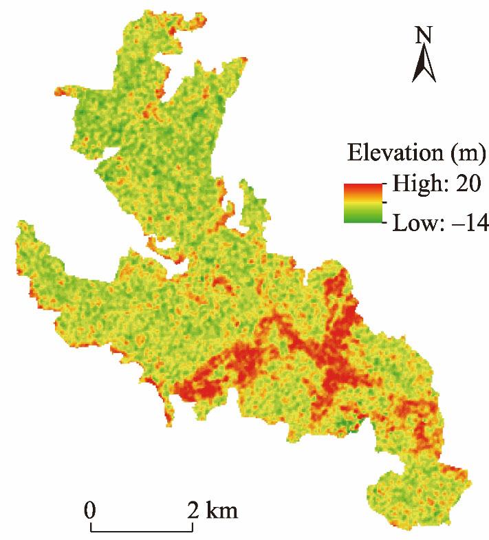
Fig. 1. Overview and elevation of New Town Kolkata.

2.2. Data sources

This study used Landsat TM, ETM+, and OLI data with 10-a intervals from 1991 to 2021 (Table 1). All Landsat and Shuttle Radar Topography Mission-Digital Elevation Model (SRTM-DEM) data were gathered from the United States Geological Survey (https://earthexplorer.usgs.gov). All referenced data were collected from Google Earth to determine the accuracy of classified images in various years. Other spatial data were collected from DIVA-GIS website (https://www.diva-gis.org/Data).
Table 1 Details about satellite data for land use/land cover (LULC) and land surface temperature (LST) analysis.
Satellite Sensor Path Spatial resolution (m) Cloud cover (%) Date Season Purpose of use
Landsat 5 TM 138/44 30 9 17 Jan 1991 Winter LST
Landsat 5 TM 138/44 30 2 6 Mar 1991 Spring LULC
Landsat 5 TM 138/44 30 33 23 Apr 1991 Summer LST
Landsat 5 TM 138/44 30 11 30 Sep 1991 Autumn LST
Landsat 7 ETM+ 138/44 30 7 4 Jan 2001 Winter LST
Landsat 5 TM 138/44 30 4 17 Mar 2001 Spring LULC
Landsat 7 ETM+ 138/44 30 0 26 Apr 2001 Summer LST
Landsat 7 ETM+ 138/44 30 11 19 Oct 2001 Autumn LST
Landsat 7 ETM+ 138/44 30 13 16 Jan 2011 Winter LST
Landsat 7 ETM+ 138/44 30 0 6 Apr 2011 Summer LST and LULC
Landsat 7 ETM+ 138/44 30 6 31 Oct 2011 Autumn LST
Landsat 8 OLI and TIRS 138/44 30 11 3 Jan 2021 Winter LST
Landsat 8 OLI and TIRS 138/44 30 0 4 Feb 2021 Spring LULC
Landsat 8 OLI and TIRS 138/44 30 0 25 Apr 2021 Summer LST
Landsat 9 OLI and TIRS 138/44 30 0 7 Nov 2021 Autumn LST

Note: TM, Thematic Mapper; ETM+, Enhanced Thematic Mapper Plus; OLI, Operational Land Imager; TIRS, Thermal Infrared Sensor.

2.3. Methods

2.3.1. Image processing

In the image processing stage, this study used the ArcGIS 10.4 software (Environmental Systems Research Institute, Redlands, the United State) for atmospheric correction, radiometric correction, composite band making, and image improvement through histogram equalization (Fig. 2).
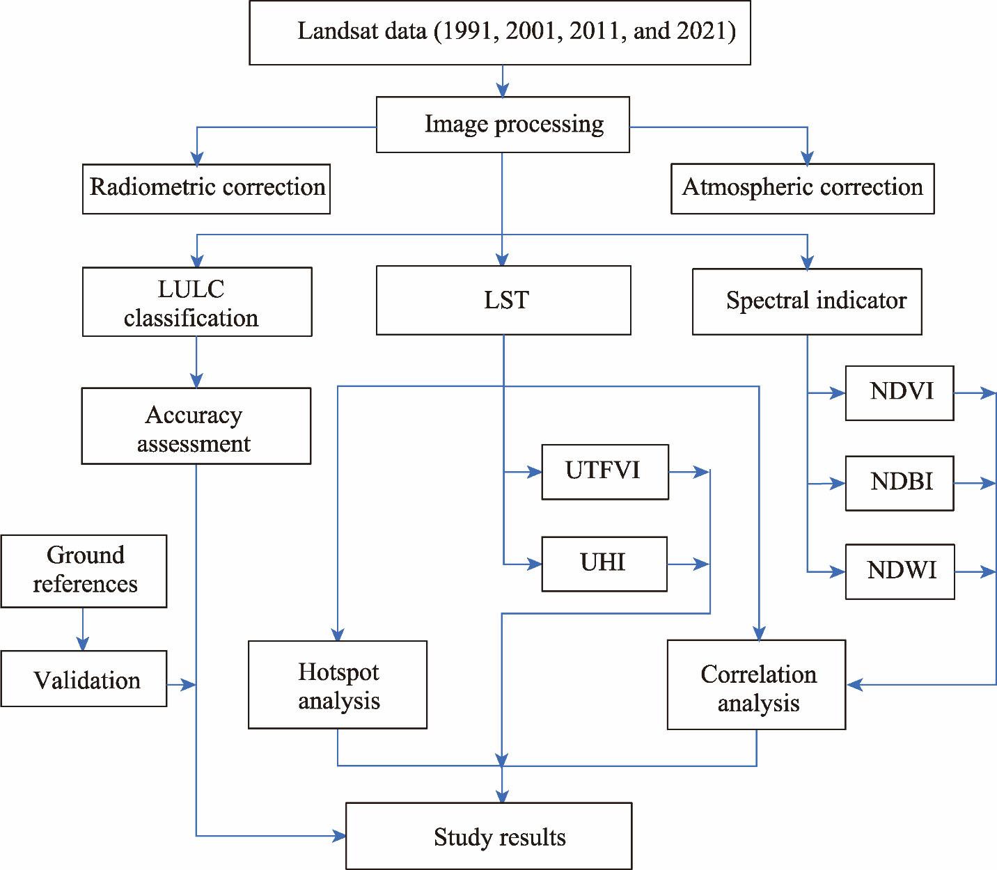
Fig. 2. Methodological flow of this study. LST, land surface temperature; LULC, land use/land cover; NDBI, normalized difference built-up index; NDVI, normalized difference vegetation index; NDWI, normalized difference water index; UHI, urban heat island; UTFVI, urban thermal field variance index.

2.3.2. Image classification

This study used the supervised maximum likelihood classification method to differentiate the types on the LULC map. In this study, six primary LULC types, including built-up land, dense vegetation, sparse vegetation, agricultural land, fallow land, and water body, were selected (Table 2). Some previous studies have chosen these as the most important parameters for studying LULC dynamics and the environmental impact (Das et al., 2021; Haldar et al., 2023; Seyam et al., 2023). The supervised maximum likelihood classification method depends upon the training sites collected from the user’s field knowledge. The first step of this method is to select the areas that will be used as training sites for image classification; then, signatures or spectral response characteristics for each LULC type are generated for the final image classification. According to earlier studies, the maximum likelihood algorithm method evaluates the normal distribution statistics of each pixel for each band; in other words, it estimates the probability that a pixel falls within a particular LULC type. For all LULC types, this probability is constant (Shalaby and Tateishi, 2007).
Table 2 Description of LULC types in this study.
LULC type Description
Built-up land Housing, roads, institutions, urban and manufacturing regions, etc.
Dense vegetation Trees with dense and confined canopy layers (Khwarahm, 2021) and vast canopies of evergreen and semi-evergreen trees planted for commercial purposes (Tarawally et al., 2019).
Sparse vegetation Areas with sparse vegetation and open canopy layers (Khwarahm, 2021), 10%-50% of the ground is covered by scattered plants, and the rest is usually bare land with meadows, immature trees, etc.
Agricultural land Land used for growing cultivated plants (Meyer and Turner, 1992).
Fallow land Unused farmland, and land with soil, sandy, rocky, or snowy condition with less than 10% natural vegetation throughout the year.
Water body Rivers, ponds, lakes, wetlands, etc.

2.3.3. Spectral indices

For a comprehensive understanding of the correlation between LULC changes and LST, several spectral indices, such as NDVI, NDBI, and NDWI, were computed using various bands of the Landsat images. Some previous studies have used these indices to analyze the relationship between LULC changes and LST (Rousta et al., 2018; Santhosh and Shilpa, 2023).
NDVI is a multi-spectral remote-sensing technique that may be applied to identify various types of vegetation coverage, classify land cover, and identify water body and vacant land (Halder et al., 2022a). In this study, NDVI was used to identify the spatiotemporal changes in the quality and quantity of vegetation. NDVI can be determined using the following equation (Das et al., 2021; Mansourmoghaddam et al., 2023a):
$NDVI=\frac{NIR-RED}{NIR+RED}$,
where NIR is the near-infrared band (µm); and RED is the red band (µm). The value of NDVI varies from -1.00 to 1.00. A value closes to -1.00 indicates a water body area, whereas that nears 1.00 indicates healthy vegetation and forest cover (Halder et al., 2021).
NDBI was applied to extract the extent of built-up land. It was obtained using the following equation (Verma and Garg, 2021):
$NDBI=\frac{SWIR-NIR}{SWIR+NIR}$,
where SWIR is the short-wave near-infrared band (µm). The value of NDBI varies between -1.00 and 1.00. A negative value of NDBI indicates the presence of water body, and the positive value represents build-up land.
NDWI is the most suitable index for mapping the water body. This study used it to identify surface water body, including ponds, lakes, rivers, and wetlands. NDWI could be calculated using the following equation (Ashwini and Sil, 2022):
$NDWI=\frac{\operatorname{NIR}-SWIR}{\operatorname{NIR}+SWIR}$.
The value of NDWI varies from -1.00 to 1.00. Usually, when the value of NDWI is greater than 0.50, it indicates water body.

2.3.4. Accuracy assessment

Accuracy assessment is very crucial for every image classification. The classified image must be compared with the referenced image that is correct or based upon ground truth data. An error matrix has been created to determine the user and producer accuracy of the supervised image classification. For the image accuracy assessment, 212 sample locations were collected from Google Earth Engine and matched with the classified image.
The user’s accuracy can be estimated by dividing the number of matched sites in a particular LULC type by the sum of the number of sites in the same type multiplied by 100 (Story and Congalton, 1986). The commission error of the user’s accuracy shows the likelihood of a site being classified in a type that it truly represents (Lunetta et al., 2006; Pal and Ziaul, 2017). The producer’s accuracy is estimated by dividing the number of matching sites by the sum of the number of sites evolved from data sets multiplied by 100. It assesses how well a region has been classified. The omission error of the producer’s accuracy is the proportion of observed locations in the field that are not identified in the referenced map.
The kappa coefficient is another important index for determining the accuracy of the image classification. Some earlier studies have used this method for image accuracy assessment (Moazzam et al., 2022; Mansourmoghaddam et al., 2023a). It can be calculated using Equations 4 and 5. When the kappa coefficient is less than 0.40, the accuracy is poor; meanwhile, that of 0.40-0.55 indicates good accuracy, that of 0.55-0.70 indicates very good accuracy, and that of 0.70-0.85 indicates exceptional accuracy.
$k=\frac{\frac{\sum{a}}{N}-\sum{\text{EF}}}{1-\sum{\text{EF}}}$,
where k denotes the kappa coefficient; a means the diagonal frequency; N represents the total number of frequencies; and EF denotes the expected frequency.
$\text{EF}=\frac{Ra{{w}_{total}}\times Colum{{n}_{total}}}{N}$,
where Rawtotal is the total number of classified pixels in a particular class; and Columntotal is the total number of reference pixels in a particular class.

2.3.5. Calculation of land surface temperature (LST)

The LST is determined by the degree of heat emitted from the Earth’s surface depending on various LULC types (Kayet et al., 2016). Thermal bands of the various Landsat series images were used to calculate the LST. Regarding Landsat OLI, it was found that band 10 was better than band 11 for finding out the LST because band 11 was much more affected by stray light (Montanaro et al., 2015). This study used band 6 of Landsat TM and ETM+ as well as band 10 of Landsat OLI for the LST calculation. ArcGIS 10.4 software was used to extract LST from Landsat thermal bands in many steps. The LST maps were generated using the following formulas.
Step 1: conversion to spectral radiance. The conversion of digital numbers to spectral radiance was performed by applying Equation 6 for Landsat 5 and 7 and Equation 7 for Landsat 8 and 9 (Guha and Govil, 2022):
${{L}_{\lambda }}=\frac{{{L}_{\max \lambda }}-{{L}_{\min \lambda }}}{QCa{{l}_{\max }}-\,QCa{{l}_{\min }}}\times (QCal-QCa{{l}_{\min }})\,+\,L{{\min }_{\lambda }}$,
where Lλ is the spectral radiance (W/(sr•m2•nm)); Lmaxλ is the maximum spectral radiance of band 6 (W/(sr•m2•nm)); Lminλ is the minimum spectral radiance of band 6 (W/(sr•m2•nm)); QCal is the quantized calibrated pixel value in digital numbers; QCalmax is the maximum quantized calibrated pixel value in digital numbers; and QCalmin is the minimum quantized calibrated pixel value in digital numbers.
${{L}_{\lambda }}=\,{{M}_{L\,}}\times QCal\,+\,{{A}_{L}}$,
where ML is the radiance multiplicative scaling factor; and AL is the radiance additive scaling factor for the thermal band.
Step 2: transformation of spectral radiance to brightness temperature. The spectral radiance was transformed into the brightness temperature by applying Equation 8 (Ramaiah et al., 2020).
$\text{BT}=\frac{{{K}_{2}}}{\text{ln}\,\left( \frac{{{K}_{1}}}{{{L}_{\lambda }}}\,+\,1 \right)}\,-273.15$,
where BT means brightness temperature (°C); and K1 and K2 denote constant bands, and the values of K1 and K2 remain constant for each satellite image.
In the case of Landsat 8 OLI, the values of K1 and K2 for band 10 were 774.8853 and 1321.0789, respectively. Additionally, for the Landsat TM, the values of K1 and K2 for band 6 were 607.7600 and 1260.5600, respectively. For the Landsat ETM+, the values of K1 and K2 for band 6 were 666.0900 and 1282.7100, respectively.
Step 3: calculation of NDVI. The proportion of vegetation was performed using Equations 1 and 9 (Haldar et al., 2023). For calculating the proportion of vegetation, the lowest and highest NDVI values were considered:
${{P}_{V}}=\,{{\left( \frac{NDVI-\,NDV{{I}_{\min }}}{NDV{{I}_{\max }}-NDV{{I}_{\min }}} \right)}^{2}}\times 100%$,
where PV means the proportion of vegetation (%); and NDVImin and NDVImax are the minimum and the maximum of NDVI, respectively.
Step 4: calculation of land surface emissivity. Equation 10 was used to compute the land surface emissivity (Avdan and Jovanovska, 2016; Halder et al., 2021):
$e=0.004\,\times \,{{P}_{V}}\,+\,0.986$,
where e means land surface emissivity.
Step 5: calculation of LST (°C) (Kumari et al., 2018).
$LST=\frac{\text{BT}}{1}+W\times \left( \frac{\text{BT}}{\text{P}} \right)\times \text{ln}\left( e \right)$,
where W means the wavelength of emitted radiance (µm); and P is a constant.

2.3.6. Urban thermal field variance index (UTFVI)

The impact of UHI has been extensively examined using the UTFVI (Tomlinson et al., 2011). The UHI phenomena are produced by various elements, including heat waves, psychometric conditions, Earth’s surface modifications, and illumination intensity (Kafy et al., 2021b). The UTFVI was computed using the following equation (Halder et al., 2021):
$UTFVI=\frac{LST-LS{{T}_{mean}}}{LS{{T}_{mean}}}$,
where LSTmean is the average LST (°C). According to the variations, we classified the UTFVI into six distinct categories: none, weak, middle, strong, stronger, and strongest.

2.3.7. Urban heat island (UHI)

The study of UHI plays a more significant role for the urban heat balance analysis (Halder et al., 2021). UHI maps were prepared to determine the status of urban thermal environment using Equation 13 (Halder et al., 2022b). The “Raster Calculator” tool available in ArcGIS 10.4 software was used to prepare the UHI and UTFVI maps.
$UHI=\frac{LST-LS{{T}_{mean}}}{SD}$,
where SD means the standard deviation of LST (°C).

2.3.8. Correlation analysis

The correlation analysis based on the Pearson’s product moment correlation coefficient (r) method was applied to obtain more knowledge of the connection between LST and various spectral indices, such as NDVI, NDBI, and NDWI (Rousta et al., 2018; Kafy et al., 2020; Santhosh and Shilpa, 2023). The correlational data were obtained using “create fishnet” and “extract multiple values to point” functions in ArcGIS10.4 software (Halder et al., 2022a). Furthermore, based on linear regression, we developed a scattered plot to increase the understanding of the relationship between LST and various spectral indices.

2.3.9. Hotspot analysis (Getis-Ord Gi* index)

This study used the Getis-Ord Gi* index, also known as hotspot analysis, to assess the intensity of LST hot spots and identify local hot and cold spots (Ding et al., 2015) using ArcGIS 10.4 software. This method can differentiate between high and low concentrations of cluster formation. For an attribute to be counted as a statistically significant hotspot, it must not only have a high value but also be surrounded by numerous other characteristics that also have high values (Tran et al., 2017; Mansourmoghaddam et al., 2023b); only then will it be considered a significant hotspot. The Getis-Ord Gi* index was computed using the following equations:
$Getis-Ord Gi*=\frac{\sum\nolimits_{j=1}^{n}{{{w}_{ij}}}{{x}_{j}}-\bar{X}\sum\nolimits_{j=1}^{n}{{{w}_{ij}}}}{\sqrt[S]{\frac{\left[ n\sum\nolimits_{j=1}^{n}{{{w}_{ij}}^{2}-\left( \sum\nolimits_{j=1}^{n}{{{w}_{ij}}} \right)} \right]}{n-1}}}$,
$\bar{X}=\frac{\sum\nolimits_{j-1}^{n}{{{x}_{j}}}}{n}$,
$S=\sqrt{\frac{\sum\nolimits_{j-1}^{n}{x_{n}^{2}}}{n}}-{{\left( {\bar{X}} \right)}^{2}}$,
where wij is the spatial weight between feature i and feature j; xj is the attribute value for feature j; $\bar{X}$ is the mean value of the features; S is the standard deviation of the features; n is the total number of features; and xn is the attribute value of the features. The Z-score is the result of the Getis-Ord Gi* index for every element. Higher positive Z-scores indicate stronger clustering of high values (hot spot), whereas smaller negative Z-scores show deeper clustering of low values (cold spot). Based on the confidence level bin (Gi_Bin), we divided the Getis-Ord Gi* index into seven distinct groups. Values with a Gi_Bin value of either 3 or -3 are statistically significance at 99% confidence level (extremely hot spot or extremely cold spot); values with a Gi_Bin value of either 2 or -2 reflect a 95% confidence level (hot spot or cold spot); values with a Gi_Bin value of either 1 or -1 reflect a 90% confidence level (whether it be a hot spot or a cold spot); and values with a Gi_Bin value of 0 are not statistically significant (Environmental Systems Research Institute, 2023). The P-value and Z-score represent the normal distribution of Getis-Ord Gi* index. If the Z-score is less than -1.65 or greater than 1.65, then P<0.10; if the Z-score is less than -1.96 or greater than 1.96, then P<0.05; finally, when the Z-score is less than -2.58 or greater than 2.58, then P<0.01 (Das and Angadi, 2020).

2.3.10. Analysis of the cooling effect of vegetation on LST

In this study, we selected two green spaces based on NDVI maps and Google Earth images. For better results, water body was excluded from the LST map. Buffer zones of 300 m distances were developed at 100 m intervals using the buffer tool in ArcGIS 10.4 software. In this study, we measured the cooling distance based on the first turning point of the curve from the green space boundary (Dong et al., 2022).

3. Results and discussion

3.1. Spatiotemporal changes in land use/land cover (LULC) during 1991-2021

The LULC changes of New Town Kolkata from 1991 to 2021 were evaluated using various Landsat images. Ultimately, six major LULC types were selected, including built-up land, dense vegetation, sparse vegetation, agricultural land, fallow land, and water body (Table 2).
In 1991, most of the study area was rural, being mostly connected with primary activities. This region was dominated by wetlands, forests, agricultural lands, and vast water bodies (Kundu, 2016). At this time, the area percentage of vegetation cover (both dense and sparse vegetation) was very high (42.80% of the total); this was followed by built-up land (21.91%), fallow land (21.01%), agricultural land (11.82%), and water body (2.46%; Table 3). The built-up land (containing mostly rural settlements) was very large in the eastern part, with significant vegetation cover in the region’s middle and southern parts (Fig. 3).
Table 3 Area changes of LULC types during 1991-2021.
LULC type 1991 2001 2011 2021
Area (km2) Percentage (%) Area (km2) Percentage (%) Area (km2) Percentage (%) Area (km2) Percentage (%)
Agricultural land 3.85 11.82 6.79 20.85 6.26 19.22 2.49 7.65
Built-up land 7.13 21.91 6.19 19.02 9.21 28.29 14.85 45.63
Dense vegetation 4.54 13.94 8.12 24.96 5.24 16.10 6.38 19.60
Fallow land 6.84 21.01 3.59 11.02 4.17 12.82 5.64 17.34
Sparse vegetation 9.40 28.86 6.44 19.78 6.04 18.54 0.92 2.82
Water body 0.80 2.46 1.42 4.37 1.63 5.02 2.28 6.99
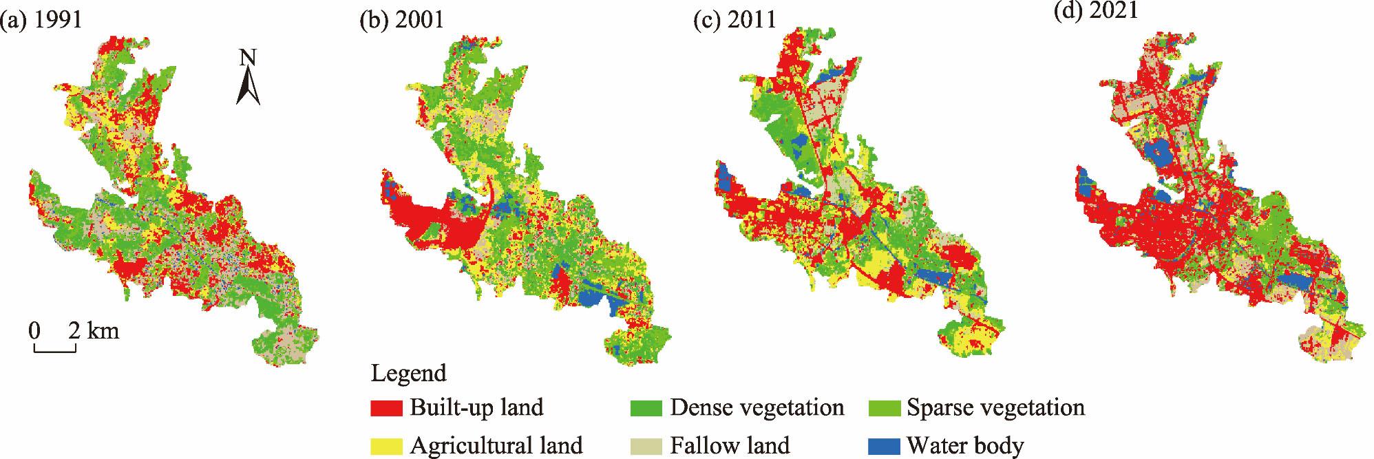
Fig. 3. Spatial distribution of LULC types in New Town Kolkata in 1991 (a), 2001 (b), 2011 (c), and 2021 (d).
After 1993, when the New Town Kolkata project began, the government occupied a large amount of land to construct urban infrastructure, which affected the local people. Mass population displacement was witnessed (Mitra and Banerji, 2018). This situation has led to a negative growth rate of built-up land (1990-2001). The area growth rate of built-up land was -13.22% from 1991 to 2001, followed by 48.80% (2001-2011) and 61.25% (2011-2021; Table 4). The construction of different types of infrastructure within the rural region has led to the rapid growth of built-up land and the loss of forest areas. The area percentage of parse vegetation decreased from 28.86% in 1991 to 2.82% in 2021 (Table 3).
Table 4 Area growth rate of different LULC types during 1991-2021.
LULC type Area growth rate during 1991-2001 (%) Area growth rate during 2001-2011 (%) Area growth rate during 2011-2021 (%)
Agricultural land 76.37 -7.79 -60.22
Built-up land -13.22 48.80 61.25
Dense vegetation 79.02 -35.48 21.68
Fallow land -47.56 16.36 35.18
Sparse vegetation -31.47 -6.20 -84.78
Water body 78.09 14.76 39.22
From 1991 to 2001, the area percentage of built-up land decreased from 21.91% to 19.02% and the area percentage of agricultural land increased from 11.82% to 20.85%. Implementation of the river-lifting irrigation scheme and the foundation of 15 pumping stations with medium capacity were completed at the Bagjola Canal (Chakrabarty et al., 2015), which has led to agricultural activities. Between 1990 and 2003, metalled roads were developed to connect the eastern metropolitan bypass and the Kaji Nazrul Islam Sarani Road with Kolkata Airport. In 2001, vegetation was improved on the eastern side due to acquired areas (rural habitation, agricultural land, etc.) left unused after development activities like earth-filling. Some vegetation patches also grew naturally there (Mitra and Banerji, 2018).
From 2001 to 2011, the government introduced several plans for the development of urban infrastructure, like transport, land development projects, an east-west corridor, a six-lane Bajgola bridge, sewerage, drainage, water supply, and sewerage pumping systems in New Town Kolkata (WBHIDCO, 2010). For that reason, the area percentage of built-up land rapidly increased from 19.02% in 2001 to 28.29% in 2011, while dense and sparse vegetation decreased (Table 3). Most of the built-up expansion could be found in the northwestern part, closer to the Kolkata City (Fig. 3).
Due to rapid urbanization, LULC changed significantly from 2011 to 2021. In 2016, under the smart city mission, the government focused on restructuring and redeveloping the city. Therefore, the area percentage of built-up land increased from 28.29% in 2011 to 45.63% in 2021. Previous report showed that urbanization has affected agricultural land significantly (Kundu, 2016). Recent plantation initiatives may have enhanced dense vegetation from 16.10% to 19.60%. The area percentage of sparse vegetation declined considerably from 18.54% to 2.82% (Table 3). This decrease can be linked to the attractiveness of real estate development.
From 2011 to 2021, various urbanization projects have been implemented. Between 2011 and 2015, sewerage, drainage, and water supply projects were completed in more than 90.00% of the study area. Several ecoparks and cultural convention centers were developed during 2011-2015 (WBHIDCO, 2015). Since 2016, various projects have been completed across the whole of New Town Kolkata, like the Biswa Bangla Convention Centre, swimming pools, and business clubs (WBHIDCO, 2023).
The area growth rates of agricultural land during 2001-2011 and 2011-2021 were -7.79% and -60.22%, respectively. Illegal infiltrations and the implementation of various development projects have forced agricultural land and vegetation coverage area to be converted into built-up land. Construction of different types of infrastructure within the rural region has led to the rapid growth of built-up land and the loss of forest areas.
Very high negative growth (-84.78%) of sparse vegetation occurred during 2011-2021 (Table 4). Fast expansion of human settlements, roadways, and illegal deforestation constitute major reasons for the loss of vegetation in this region. The area percentage of water body has continuously increased from 2.46% in 1991 to 6.99% in 2021 (Table 3). From the above analysis, we can find that urbanization and population expansion may soon be a significant concern for urban planners. Therefore, proper LULC management should be followed.

3.1.1. Land conversion during 1991-2021

From 1991 to 2021, New Town Kolkata witnessed various township projects. These township projects and the resultant rapid urbanization promoted land conversion and LULC changes, as shown in Table 5 and Figure 4. Table 5 shows that built-up land has increased and exhibited the foremost positive change. In contrast, sparse vegetation has changed drastically due to its conversion into other LULC types, such as built-up land (4.13 km2), fallow land (1.70 km2), dense vegetation (1.72 km2), agricultural land (0.74 km2), and water body (0.85 km2). Reverse transfer from built-up land to sparse vegetation, dense vegetation, and agricultural land promotes environmental sustainability. Land acquisition, displacement of people, and the impact of various projects may be the cause of land conversion. After 2016, the smart city mission in New Town Kolkata changed the city’s morphology.
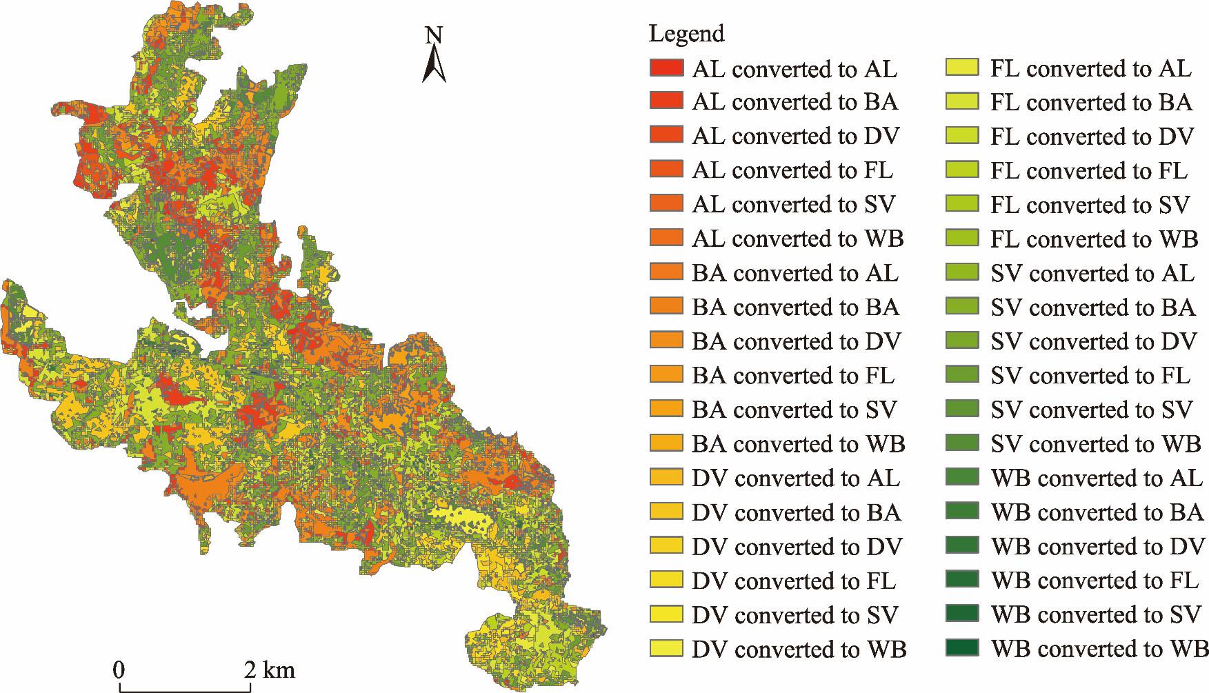
Fig. 4. Land conversion of various LULC types during 1991-2021. AL, agricultural land; BA, built-up land; DV, dense vegetation; FL, fallow land; SV, sparse vegetation; WB, water body.
Table 5 LULC conversion matrix during 1991-2021.
LULC type Agricultural land (km2) Built-up land (km2) Dense vegetation (km2) Fallow land (km2) Sparse vegetation (km2) Water body (km2) Total area in 1991 (km2) Area loss (km2)
Agricultural land 0.24 1.99 0.72 0.69 0.06 0.15 3.85 -3.61
Built-up land 0.48 3.29 1.64 1.06 0.41 0.25 7.13 -3.84
Dense vegetation 0.47 2.22 0.26 0.93 0.07 0.59 4.54 -4.28
Fallow land 0.53 2.87 1.79 1.18 0.11 0.36 6.84 -5.66
Sparse vegetation 0.74 4.13 1.72 1.70 0.26 0.85 9.40 -9.14
Water body 0.03 0.35 0.25 0.08 0.01 0.08 0.80 -0.72
Total area in 2021 (km2) 2.49 14.85 6.38 5.64 0.92 2.28
Area gain (km2) 2.25 11.56 6.12 4.46 0.66 2.20

3.1.2. Accuracy assessment of the LULC classification

This study used user’s accuracy, producer’s accuracy, overall accuracy, and kappa coefficient for accuracy assessment purposes. The overall accuracy of all classified images was 95.45%, 94.11%, 93.55%, and 92.73% for 1991, 2001, 2011, and 2021, respectively, indicating a very high accuracy level. The kappa coefficient for all classified images was 0.9379 for 1991, 0.9285 for 2001, 0.9222 for 2011, and 0.9122 for 2021. Thus, the overall accuracy and kappa coefficients are acceptable.

3.2. Spatial pattern of normalized difference vegetation index (NDVI), normalized difference built-up index (NDBI), and normalized difference water index (NDWI) during 1991-2021

In 1991, the NDVI values varied from -0.18 to 0.47. A high NDVI value (>0.40) was recorded in the middle part of this region, indicating the presence of healthy vegetation. In 2021, the NDVI values had improved, ranging from -0.07 to 0.40 again in the middle part of the region (Fig. 5). The extent and health condition of vegetation varied over time. NDBI reveals the extent of impermeable built-up land in this region, as a greater NDBI value is associated with more such surfaces. Our assessment revealed that NDBI dynamically changed from 1991 to 2011 (Fig. 5). A trend toward sustainable land use strategies like urban agriculture or green infrastructure may explain the declining NDBI value in 2021. The smart city project reconstructed and redeveloped the city. There are a few exceptions to the association between NDVI and NDBI; for instance, NDVI can be high in cities with extensive parks or green areas even though there is still significant densely built-up land nearby. NDWI presents both the availability of water and its concentration in a region (Haldar et al., 2023). NDWI value has significantly increased since 1991, indicating that water body in this region has increased.
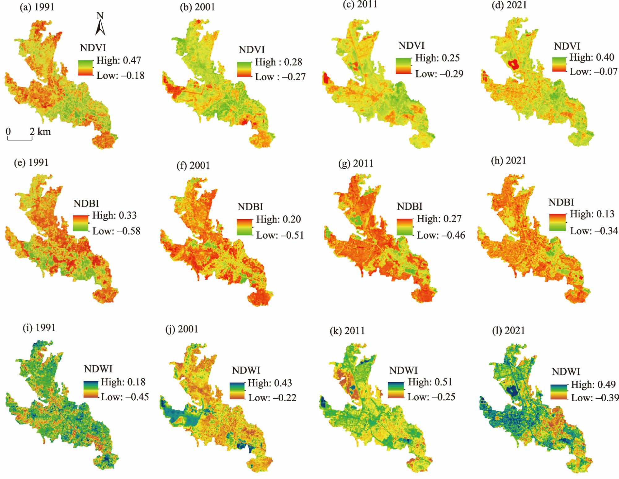
Fig. 5. Spatiotemporal changes of NDVI (a, b, c, and d), NDBI (e, f, g, and h), and NDWI (i, j, k, and l) in New Town Kolkata in 1991, 2001, 2011, and 2021.

3.3. Spatiotemporal variations of LST

The spatiotemporal variations of LST during 1991-2021 were calculated from Landsat thermal bands after applying several formulas for winter (December-February), summer (March-May), and Autumn (October-November) (Table 6). Temperatures in various parts of this region varied significantly due to urbanization. In 1991, the maximum and minimum temperatures in this region were 18.39°C and 10.93°C, respectively, in winter; 32.87°C and 23.26°C, respectively, in summer; and 21.07°C and 15.18°C, respectively, in autumn.
Table 6 Seasonal variations of LST during 1991-2021.
LST in winter 1991 2001 2011 2021
Max (°C) 18.39 21.82 23.36 26.01
Min (°C) 10.93 16.55 16.55 18.57
Mean (°C) 16.31 18.98 20.59 22.48
SD (°C) 0.87 0.76 1.23 1.21
CV (%) 5.31 4.01 5.97 5.36
LST in summer 1991 2001 2011 2021
Max (°C) 32.87 36.40 34.55 39.62
Min (°C) 23.26 25.87 23.86 27.66
Mean (°C) 29.18 30.10 29.31 34.61
SD (°C) 1.44 1.64 1.95 1.84
CV (%) 4.95 5.45 6.65 5.31
LST in autumn 1991 2001 2011 2021
Max (°C) 21.07 26.87 28.30 30.58
Min (°C) 15.18 20.27 19.62 24.19
Mean (°C) 19.18 24.02 23.29 27.11
SD (°C) 0.84 1.23 1.30 1.01
CV (%) 4.36 5.11 5.60 3.73

Note: Max, maximum; Min, minimum; SD, standard deviation; CV, coefficient of variation.

The spatiotemporal variations of LST were characterized by rapid changes of LULC due to several stages of urbanization, including the planning of the new town and land acquisition (1991-2006), displacement of people (1991-2011), the smart city initiative (2016), and city restructuring and development (2017-present).
The dynamic nature of LULC has impacted the temporal variations of LST. The mean temperature in winter increased significantly from 16.31°C to 22.48°C during 1991-2021. In summer and autumn, the mean temperature significantly increased from 29.18°C to 34.61°C and 19.18°C to 27.11°C, respectively (Table 6). There was no significant difference in mean temperature between 2001 and 2011, except for some earlier patches being more intense and some new high-temperature patches recorded in numerous portions of the study area.
The higher temperatures in this area are shown in Figure 6 in red color, while the lower temperatures are shown in blue color. The area with higher temperatures has changed every decade due to ongoing dynamic urbanization. However, some parts of the area, like the western, northern, and northeastern parts, have remained located in the high-temperature zone. As these parts are adjacent to Kolkata City, the density of build-up land is high, and the presence of open spaces and vegetation is low. It can be expected that LST will increase in the future.
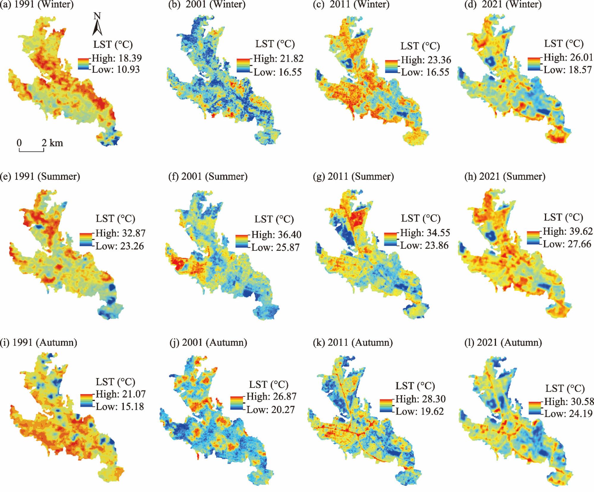
Fig. 6. Spatiotemporal variations of LST in winter (a, b, c, and d), summer (e, f, g, and h), and autumn (i, j, k, and l) in 1991, 2001, 2011, and 2021.
From 1991 to 2021, the significant differences of the maximum, minimum, and mean temperatures in summer were 6.75°C, 4.40°C, and 5.43°C, respectively; in winter, they were 7.62°C, 7.64°C, and 6.17°C, respectively; and in autumn, they were 9.51°C, 9.01°C, and 7.93°C, respectively. In all seasons, the mean LST increased above 5.00°C (Table 6); this reveals that the vast dynamic change of the natural environment, especially vegetation and cultivated land, to built-up land may be responsible for increasing LST.
Overall, LST increased seasonally, which is alarming. Declining forest cover, surface water body, unplanned urbanization, and climate change may all lead to a rising trend in LST.

3.4. Spatiotemporal changes of LST in various LULC types during 1991-2021

The mean LST for all LULC types was calculated using ArcGIS 10.4 software. Due to different rates of radiated energy from the Earth’s surface, vegetation, farmlands, barren lands, building roofs, impermeable surfaces, and surface water body have different LSTs (Voogt and Oke, 2003). Cemented built-up areas contribute to higher temperatures, whereas vegetation-covered areas have a strong role in reducing LST and provide cooling effects on the urban environment (Grover and Singh, 2015).
From 1991 to 2021, in summer, the mean LST of built-up land rose from 30.04°C to 35.14°C, while the mean LST of fallow land increased from 28.91°C to 35.60°C. The mean LST of other LULC types like agricultural land, dense vegetation, sparse vegetation, and water body increased from 30.33°C to 35.18°C, 28.27°C to 33.71°C, 28.72°C to 33.68°C, and 28.72°C to 31.20°C, respectively. In winter, the mean LST of built-up land increased from 20.80°C to 22.67°C; conversely, the mean LST of agricultural land, water body, and fallow land increased from 20.70°C to 23.28°C, 20.14°C to 20.68°C, and 20.22°C to 23.40°C, respectively, as shown in Table 7.
Table 7 Spatiotemporal changes of LST across various LULC types during 1991-2021.
LULC type LST in summer of 1991 LST in winter of 1991
Max (°C) Min (°C) Mean (°C) SD (°C) Max (°C) Min (°C) Mean (°C) SD (°C)
Agricultural land 32.87 23.25 30.33 1.29 22.38 14.24 20.70 0.96
Built-up land 32.87 23.26 30.04 1.27 22.82 14.71 20.80 0.81
Dense vegetation 31.24 23.69 28.27 1.05 21.51 11.40 19.77 1.02
Sparse vegetation 32.06 23.25 28.72 1.13 21.94 10.92 20.05 1.04
Water body 31.24 23.25 28.72 1.11 21.94 13.78 20.14 0.94
Fallow land 32.87 23.25 28.91 1.48 21.94 11.88 20.22 1.00
LST in summer of 2001 LST in winter of 2001
Max (°C) Min (°C) Mean (°C) SD (°C) Max (°C) Min (°C) Mean (°C) SD (°C)
Agricultural land 33.60 27.36 30.65 1.04 21.82 17.09 19.23 0.75
Built-up land 36.39 27.36 31.83 1.63 21.82 17.09 19.19 0.71
Dense vegetation 32.19 26.37 29.28 0.90 21.82 16.55 18.66 0.68
Sparse vegetation 32.19 26.37 28.88 1.13 21.82 17.09 19.21 0.70
Water body 30.76 25.87 27.66 0.92 20.78 17.09 18.32 0.69
Fallow land 34.54 27.36 31.06 0.95 21.82 17.09 18.80 0.67
LST in summer of 2011 LST in winter of 2011
Max (°C) Min (°C) Mean (°C) SD (°C) Max (°C) Min (°C) Mean (°C) SD (°C)
Agricultural land 34.07 26.87 30.09 0.91 23.36 18.16 21.45 0.68
Built-up land 34.55 24.87 30.26 1.42 23.36 17.09 20.94 0.99
Dense vegetation 32.19 24.36 27.09 1.28 22.33 16.55 19.62 0.86
Sparse vegetation 33.60 24.36 28.74 1.43 23.36 16.55 20.29 1.05
Water body 30.76 23.86 26.23 1.20 22.84 16.55 18.39 1.07
Fallow land 34.54 24.87 30.86 1.65 23.36 17.62 21.05 1.05
LST in summer of 2021 LST in winter of 2021
Max (°C) Min (°C) Mean (°C) SD (°C) Max (°C) Min (°C) Mean (°C) SD (°C)
Agricultural land 38.95 30.53 35.18 1.52 25.43 19.68 23.28 1.02
Built-up land 39.62 29.34 35.14 1.24 26.01 19.44 22.67 0.95
Dense vegetation 37.98 28.49 33.71 1.29 24.56 19.38 21.73 0.81
Sparse vegetation 36.64 28.54 33.68 1.40 23.89 19.59 21.22 0.73
Water body 37.15 27.65 31.20 2.34 23.96 18.56 20.68 1.04
Fallow land 39.30 29.60 35.60 1.47 25.80 19.67 23.40 0.89
The mean LST of each LULC type increased in both winter and summer during the study period. However, the mean LST of each LULC type in summer of 2011 and winter of 2001 was slightly lower than that in previous decades. Weather changes or mixed LULC trends may reduce LSTs (Grover and Singh, 2015). In addition, each LULC type in 2021 was substantially warmer than that in previous years. LST was higher in built-up land and fallow land due to high heat absorption and lower albedo; their exposed rocky surfaces absorb heat quickly and release it slowly, resulting in higher temperatures (Shahfahad et al., 2022). This study discovered that agricultural land has high levels of LST throughout the summer season, when agricultural land is left as fallow land.
Table 7 also presents mean LST of each LULC type from 1991 to 2021. The LST rose slightly across LULC types in winter. Notably, LST has risen significantly across various LULC types in summer, especially in built-up land, fallow land, and agricultural land. From 1991 to 2011, the water body’s temperature gradually decreased, maybe due to increased vegetation cover near water body. However, water surface temperatures rose significantly between 2011 and 2021. Increased concrete infrastructure in the watershed may explain this. After the smart city project initiative, infrastructures such as water parks and swimming pools were developed to beautify the watershed area.
Table 8 shows LST levels in the study area from 1991 to 2021. In 2021, 46.17% (15.04 km2) of the study area experienced temperatures between 35.00°C and 40.00°C, compared with 0.00% in 2011, 0.43% in 2001, and 0.00% in 1991. Moreover, 32.53% (10.60 km2) of the study area experienced temperatures of 30.00°C-35.00°C in 1991, which rose to 48.36% (15.75 km2) in 2001, decreased to 39.36% (12.82 km2) in 2011, and increased to 50.84% (16.56 km2) in 2021. In 2021, 50.84% and 46.17% of the study area experienced temperatures of 30.00°C-35.00°C and 35.00°C-40.00°C, respectively. This scenario predicts a sharp increase in LST of the study area, which represents a big challenge for town planners (Kafy et al., 2021c).
Table 8 Areas under the various levels of LST during 1991-2021.
LST (°C) 1991 2001 2011 2021
Area (km2) Percentage (%) Area (km2) Percentage (%) Area (km2) Percentage (%) Area (km2) Percentage (%)
20.00-25.00 0.41 1.27 0.00 0.00 0.75 2.31 0.00 0.00
25.00-30.00 21.56 66.19 16.68 51.21 19.00 58.33 0.98 3.00
30.00-35.00 10.60 32.53 15.75 48.36 12.82 39.36 16.56 50.84
35.00-40.00 0.00 0.00 0.14 0.43 0.00 0.00 15.04 46.17

3.5. Correlation between various spectral indices and LST

The strength of the relationship between various spectral indices and LST was determined with the help of ArcGIS 10.4 software (Table 9). There was a positive relationship between LST and NDBI (Fig. 7). Meanwhile, LST and NDVI showed a negative correlation (Fig. 8). Destruction of vegetation has led to enormous temperature variations in the study area. This study witnessed a weak positive correlation between LST and NDWI from 1991 to 2021. A similar result was found in the study conducted by Guha and Govil (2022). This finding may indicate the presence of water body in the urbanized areas or the construction of concrete infrastructure in water body. This study also found a positive correlation between NDBI and NDWI, indicating the possibility of concrete infrastructure in the wetlands (Ogashawara and Bastos, 2012).
Table 9 Correlation between various spectral indicators (including NDVI, NDMI and NDWI) and LST in 1991, 2001, 2011, and 2021.
1991
LST NDVI NDBI NDWI
LST 1.000 -0.017 0.426** 0.027
NDVI -0.017 1.000 -0.630** -0.949**
NDBI 0.426** -0.630** 1.000 0.472**
NDWI 0.027 -0.949** 0.472** 1.000
2001
LST NDVI NDBI NDWI
LST 1.000 -0.520** 0.845** 0.320**
NDVI -0.520** 1.000 -0.653** -0.945**
NDBI 0.845** -0.653** 1.000 0.418**
NDWI 0.320** -0.945** 0.418** 1.000
2011
LST NDVI NDBI NDWI
LST 1.000 -0.472** 0.804** 0.305**
NDVI -0.472** 1.000 -0.576** -0.964**
NDBI 0.804** -0.576** 1.000 0.387**
NDWI 0.305** -0.964** 0.387** 1.000
2021
LST NDVI NDBI NDWI
LST 1.000 -0.047 0.697** -0.132**
NDVI -0.047 1.000 -0.385** -0.965**
NDBI 0.697** -0.385** 1.000 0.181**
NDWI -0.132** -0.965** 0.181** 1.000

Note: **, correlation is significant at P<0.01 level (two-tailed).

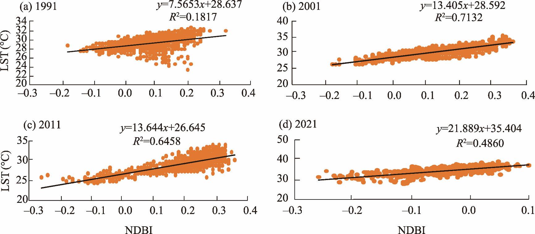
Fig. 7. Correlation between LST and NDBI in 1991 (a), 2001 (b), 2011 (c), and 2021 (d).
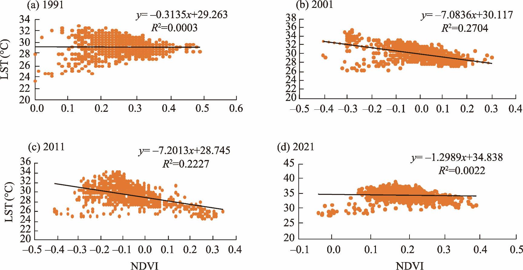
Fig. 8. Correlation between LST and NDVI in 1991 (a), 2001 (b), 2011 (c), and 2021 (d).
This study found a strong negative connection between NDVI and NDBI during the same study period, indicating that urbanization degrades vegetation. A substantial negative relationship was identified between NDVI and NDWI throughout the same study period. Rahaman et al. (2020) recorded similar results between NDVI and NDWI. In the case of a correlation between LST and NDBI, the coefficient of determination (R2) value significantly increased from 0.1817 in 1991 to 0.7132 in 2001 (Fig. 7). After 2001, the R2 value slowly decreased from 0.6458 in 2011 to 0.4860 in 2021. Overall, this indicates that, after 1991, the control of NDBI on LST increased. The R2 values between LST and NDVI were 0.0003 in 1991, 0.2704 in 2001, 0.2227 in 2011, and 0.0022 in 2021, indicating a limited influence of NDVI on LST (Fig. 8).

3.6. UTFVI and UHI analysis

UTFVI was used in this study to provide a quantitative analysis of the influence of UHI on ecological degradation. In terms of the ecological evaluation index (Table 10), according to UTFVI value, we found that poor ecological conditions were present on the western side of the map in 2001, the northern part of the map in 2011, and the middle part of the map across a small area in 2021 (Fig. 9). The change in UHI location every decade may be due to LULC changes. According to the scale of the UTFVI value (Table 10), a strong UHI was found on the western side of the study area in 2001 but the northern side of the study area in 2011.
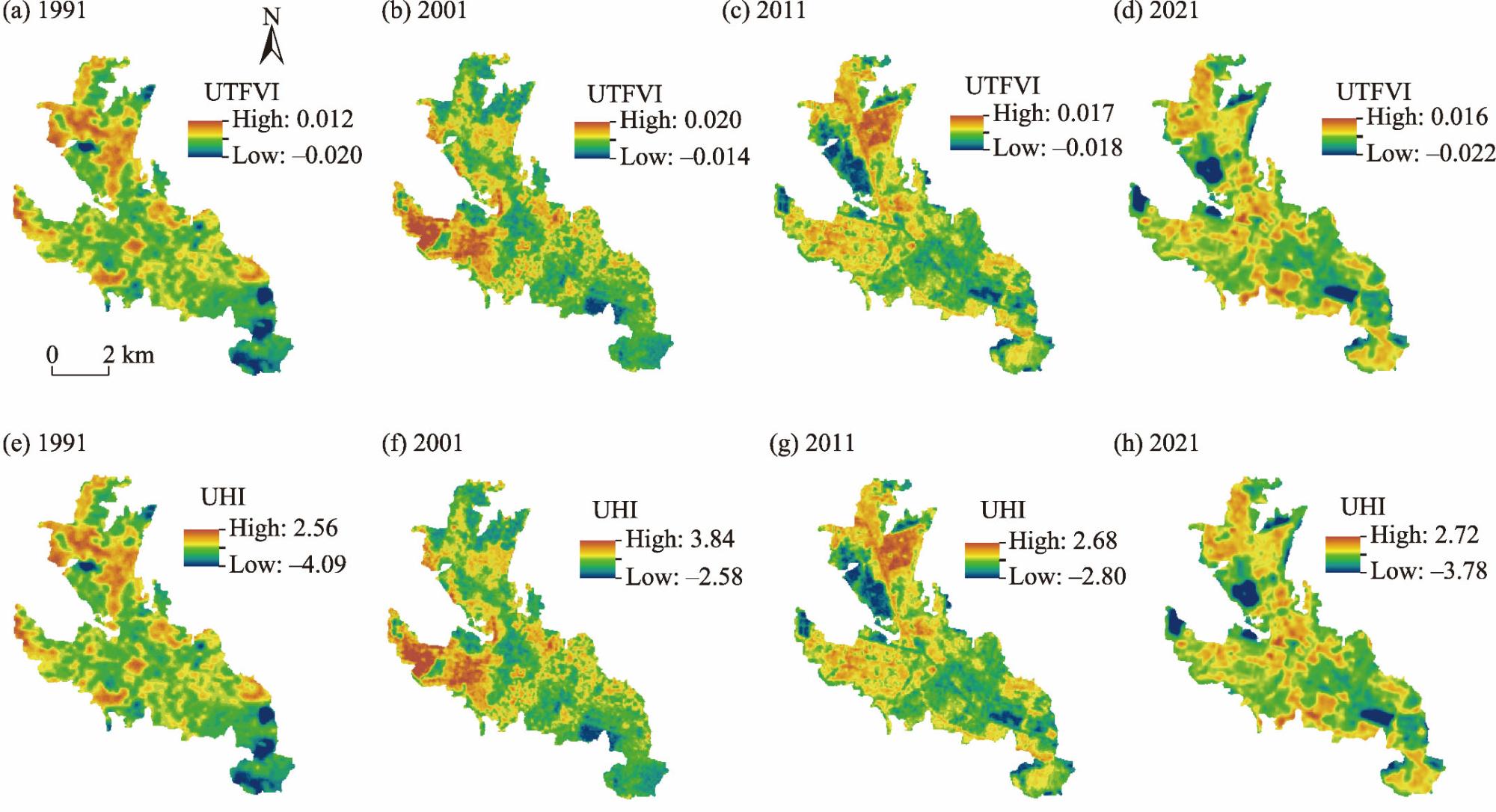
Table 10 Pattern of urban thermal field variance index (UTFVI) scale.
UTFVI value UHI phenomenon Ecological evaluation index
<0.000 None Excellent
0.000-0.005 Weak Good
0.005-0.010 Middle Normal
0.010-0.015 Strong Bad
0.015-0.020 Stronger Worse
>0.020 Strongest Worst

Note: UHI, urban heat island.

Fig. 9. Spatiotemporal distributions of UTFVI (a, b, c, and d) and UHI (e, f, g, and h) in New Town Kolkata in 1991, 2001, 2011, and 2021.
In 2021, a strong UHI was found in the middle part of the study area. High-density built-up areas have poor ecological conditions. Vegetation and water body have good ecological conditions. Various smart city projects may have reduced the heat island intensity; however, middle-type UHI was still spotted throughout a broad area of this smart city (Fig. 9). Different mitigation strategies should be taken to reduce or control them.

3.7. Hot spot and cold spot analysis

Getis-Ord Gi* index has been extensively used to identify hot spots in various research fields. This approach was employed in this study to evaluate how LULC changes affected the UHI. It might help to clarify the UHI effect on the city. The season-wise spatiotemporal patterns of hot spots and cold spots of LST during 1991 to 2021 are shown in Figure 10. Hot spot regions were found in areas saturated with roads and buildings. Cold spots were found in areas saturated with vegetation and water body.
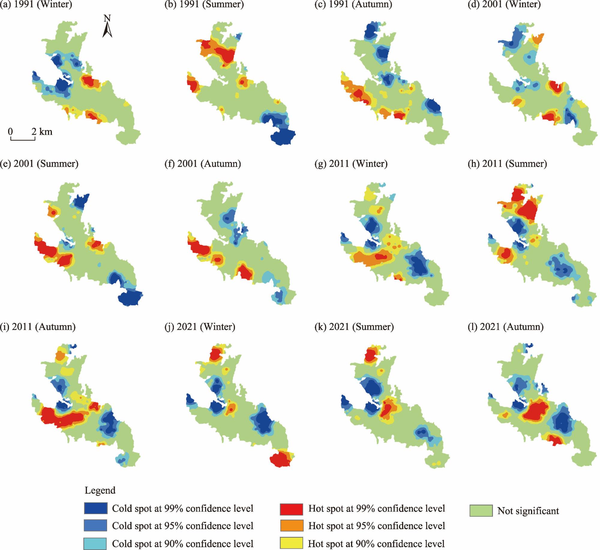
Fig. 10. Spatiotemporal distributions of hot spots and cold spots at various confidence levels in winter (a, d, g, and j), summer (b, e, h, and k), and autumn (c, f, i, and l) in New Town Kolkata in 1991, 2001, 2011, and 2021.
To examine the dynamics of hot spots and cold spots in the study area, we demonstrated a normalized distribution pattern (0.00-100.00) of hot spot and cold spot values according to 90%, 95%, and 99% confidence levels in Table 11.
Table 11 Hot spot and cold spot areas at various confidence levels in winter, summer, and autumn.
Categories Percentage of area in winter (%) Percentage of area in summer (%) Percentage of area in autumn (%)
1991 2001 2011 2021 1991 2001 2011 2021 1991 2001 2011 2021
CS (99%) 4.37 1.08 6.64 9.31 8.69 10.01 3.26 7.12 7.09 0.41 5.17 6.35
CS (95%) 5.49 7.75 7.91 5.40 3.66 3.35 8.81 6.38 6.06 5.89 7.80 8.89
CS (90%) 9.71 13.64 9.35 7.58 2.80 5.78 11.15 7.64 8.21 11.88 9.02 10.97
HS (90%) 7.02 6.94 14.90 6.62 8.06 6.74 8.23 7.42 8.72 5.82 12.37 6.36
HS (95%) 4.10 4.93 9.23 3.76 8.40 6.06 8.13 4.62 8.22 4.03 6.00 3.87
HS (99%) 2.28 3.10 1.34 6.61 6.95 8.02 9.24 3.62 2.80 6.87 10.45 7.21
NS 67.03 62.57 50.62 60.72 61.42 60.03 51.19 63.21 58.90 65.11 49.19 56.35

Note: CS (99%), cold spot at 99% confidence level; CS (95%), cold spot at 95% confidence level; CS (90%), cold spot at 90% confidence level; HS (99%), hot spot at 99% confidence level; HS (95%), hot spot at 95% confidence level; HS (90%), hot spot at 90% confidence level; NS, not significant.

In New Town Kolkata, the distribution results in summer showed that hot spots at 99%, 95%, and 90% confidence levels were observed in 6.95%, 8.40%, and 8.06% of the study area in 1991, respectively, before slightly increasing to 9.24% and 8.23% of the study area in 2011 (99% and 90% confidence levels, respectively). Then, in 2021, hot spots at 99%, 95%, and 90% confidence levels decreased to 3.62%, 4.62%, and 7.42% of the study area, respectively. The distribution results in autumn showed that hot spots at 99%, 95%, and 90% confidence levels were observed in 2.80%, 8.22%, and 8.72% of the study area in 1991, respectively, before slightly increasing to 10.45% and 12.37% of the study area in 2011 (99% and 90% confidence levels, respectively). In 2021, hot spots at 99%, 95%, and 90% confidence levels moderately decreased to 7.21%, 3.87%, and 6.36% of the study area, respectively.
The distribution results in summer showed that cold spots at 99% confidence level were observed in 8.69% of the study area in 1991, before decreasing to 3.26% of the study area in 2011. Then, in 2021, cold spots at 99% confidence level increased to 7.12% of the study area. The distribution results in autumn showed that cold spots at 99%, 95%, and 90% confidence levels were observed in 7.09%, 6.06%, and 8.21% of the study area in 1991, respectively, before increasing to 7.80% and 9.02% of the study area in 2011 (95% and 90% confidence levels, respectively). Then, in 2021, cold spots at 99%, 95%, and 90% confidence levels increased to 6.35%, 8.89%, and 10.97% of the study area respectively. Overall, after 2011, this study area witnessed a decreasing trend in hot spots and an increasing trend in cold spots, which may be related to smart city project authorities’ massive plantation campaigns and water body restoration. Despite having a high LST in 2021, this study found that the decreasing trend of hot spots due to various types of activities under the smart city project has helped to reduce the formation of high-temperature clusters. The hot spots and cold spots shifted their locations every decade, which might have been caused by random changes in the LULC patterns in this study area.

3.8. Cooling effect of vegetation on LST

Numerous earlier studies have concentrated on how green space might reduce the UHI effect in surrounding areas (Ghosh and Das, 2018; Bera et al., 2021; Dong et al., 2022; Wang et al., 2023). This study also attempts to discern the significance of green space in mitigating the UHI effect. The water body was excluded from the LST map for a better result. Buffer zones of 300 m from the edge of green space were created with an interval of 100 m, and temperature gradient graphs were constructed to show the changing pattern of temperature from the edge of green space toward its periphery. In this study, we selected two green space samples for every year. Sample 1 and Sample 2 of 2021 showed that the temperature from the edge of the green space to the 100 m buffer zone decreased by 1.53°C and 1.97°C, respectively. Also, Sample 1 and Sample 2 of 2011 showed that the temperature from the edge of the green space to the 100-m buffer zone increased by 1.27°C and 1.20°C, respectively. Here, the 0-100 m buffer zone experienced a very high rise in temperature from the mean temperature of green space compared with other buffer zones. In a few cases, the 200-300 m buffer zone showed a decreasing temperature trend, which may be the impact of outside green space (Fig. 11; Table 12). Smart city projects may be responsible for this trend, which also suggests that green space is essential to reducing the influence of the UHI effect on surrounding areas.
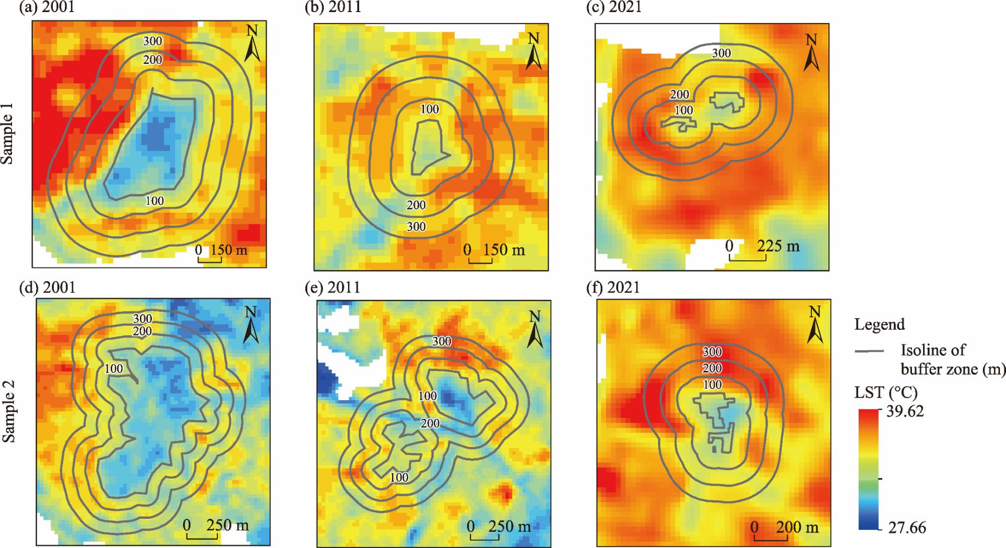
Fig. 11. Mean LST of various buffer zones from two selected green spaces in 2001, 2011, and 2021. (a, b, and c), Sample 1; (d, e, and f), Sample 2.
Table 12 LST changing pattern for each 100 m buffer zone for selected green space in 2001, 2011, and 2021.
Green space Area of green space (m2) Average LST of green space (°C) Average LST for 0-100 m buffer zone (°C) Average LST for 100-200 m buffer zone (°C) Average LST for 200-300 m buffer zone (°C) Cooling distance (m)
2001
Sample 1 175,070.00 28.94 31.53 32.67 32.60 82
Sample 2 648,622.00 29.14 30.85 31.27 31.29 56
2011
Sample 1 261,901.08 28.93 30.20 30.55 30.42 117
Sample 2 27,425.20 29.87 31.07 31.57 31.30 30
2021
Sample 1 25,110.87 34.06 35.59 36.60 36.30 138
Sample 2 36,209.57 33.12 35.09 36.15 36.45 60

4. Conclusions

Rapid urbanization can influence the urban climate and environment. After 1993, the government of West Bengal took several initiatives to develop New Town Kolkata as a planned city, which has led to significant LULC changes. The main aim of this study was to investigate the impact of LULC changes on LST from 1991 to 2021.
Regarding LULC dynamics from 1991 to 2021, this study revealed a high decline rate of area percentage of sparse vegetation from 28.86% in 1991 to 2.82% in 2021, while the area percentage of built-up land grew from 21.91% to 45.63%. This study also found a strong positive change in built-up land and a significant negative change in sparse vegetation. Negative land transfers, such as sparse vegetation converted to built-up land (4.13 km2), fallow land converted to built-up land (2.87 km2), and dense vegetation converted to built-up land (2.22 km2), may cause urban environmental issues.
This study found that, due to rapid urbanization and LULC changes, the mean temperature significantly increased from 16.31°C to 22.48°C in winter, 29.18°C to 34.61°C in summer, and 19.18°C to 27.11°C in autumn. Built-up land has experienced the maximum temperature in all periods, followed by fallow land and agricultural land. In 2021, 50.84% and 46.17% of the study area experienced temperatures in the ranges of 35.00°C-40.00°C and 30.00°C-35.00°C, respectively, which are significantly higher than those in previous years. In this study, LST and NDBI were positively associated, showing that the area of impervious surface has increased; thus, LST has also increased. LST and NDVI were negatively correlated due to plants’ cooling effect on LST. In this study, NDVI and NDBI were negatively correlated, indicating that urbanization has affected vegetation significantly. A positive correlation between NDBI and NDWI reflected concrete infrastructure in water body. This study also found that the UHI effect is more evident in dense urban than in rural or suburban regions. Poor ecological status was found in the high-density built-up areas. Excellent ecological status was found in sparse vegetation, dense vegetation, and water body. After 2011, the study area witnessed a decreasing trend of hot spots and an increasing trend of cold spots. The extensive plantation and rejuvenation of water body under the smart city project may be the cause. The hot spot and cold spot areas shifted every decade, possibly due to random LULC pattern variations. This study has some limitations: first, the low spatial resolution of Landsat images; and second, the unavailability of data for a particular time due to the high temporal frequency of Landsat images. Despite these drawbacks, the findings of this investigation will be helpful to the urban planners for sustainable urban development.
According to this study, high LST was found in this city after its emergence as a smart city. This can hamper the urban environment in the future and adversely affect human health. Therefore, proper planning is required for small towns and cities to reduce LST. Creating urban green belts, rooftop gardening, and the maintenance of roadside plantations are needed for urban sustainability. The development should be in such a way that maintains a balance between LULC changes and sustainability. In the future, policy-makers and urban planners can reduce UHI effects and create eco-friendly and sustainable smart cities based on the results of this study.

Authorship contribution statement

Bubun MAHATA: conceptualization, investigation, data curation, formal analysis, methodology, data presentation, software analysis, writing - original draft, and writing- review & editing; Siba Sankar SAHU: resources, supervision, writing - original draft, writing - review & editing, and validation; Archishman SARDAR: conceptualization, methodology, writing - original draft, and writing - review & editing; Laxmikanta RANA: conceptualization, methodology, writing - original draft, and writing - review & editing; and Mukul MAITY: conceptualization, formal analysis, methodology, data presentation, software analysis, writing - original draft, and writing - review & editing. All authors approved this manuscript.

Declaration of conflict of interest

The authors declare that they have no known competing financial interests or personal relationships that could have appeared to influence the work reported in this paper.

The first author would like to thank the University Grants Commission, New Delhi, India, for providing financial support in the form of the Junior Research Fellowship. The authors thank the United States Geological Survey (USGS) for making available Landsat 5, 7, 8, and 9 satellite images, which were downloaded from the Earth Explorer.

[1]
Ara S., Alif M.A.U.J., Islam K.M.A., et al., 2021. Impact of tourism on LULC and LST in a coastal island of Bangladesh: A geospatial approach on St. Martin’s Island of Bay of Bengal. J. Indian Soc. Remote Sens. 49(10), 2329-2345.

[2]
Ashwini K., Sil B.S., 2022. Impacts of land use and land cover changes on land surface temperature over Cachar Region, Northeast India—A case study. Sustainability. 14(21), 14087, doi: 10.3390/su142114087.

[3]
Avdan U., Jovanovska G., 2016. Algorithm for automated mapping of land surface temperature using LANDSAT 8 satellite data. J. Sens. 2016, 1480307, doi: 10.1155/2016/1480307.

[4]
Bajani S., Das D., 2020. Sustainable planning interventions in tropical climate for urban heat island mitigation—Case study of Kolkata. In: GhoshM., (ed.). Perception, Design and Ecology of the Built Environment. Cham: Springer, 167-182.

[5]
Basu T., Das A., 2023. Urbanization induced degradation of urban green space and its association to the land surface temperature in a medium-class city in India. Sustain. Cities Soc. 90, 104373, doi: 10.1016/j.scs.2022.104373.

[6]
Bera B., Shit P.K., Saha S., et al., 2021. Exploratory analysis of cooling effect of urban wetlands on Kolkata metropolitan city region, eastern India. Curr. Res. Environ. Sustain. 3, 100066, doi: 10.1016/j.crsust.2021.100066.

[7]
Bhat P.A., ul Shafiq M., Mir A.A., et al., 2017. Urban sprawl and its impact on land use/land cover dynamics of Dehradun City, India. Int. J. Sustain. Built Environ. 6(2), 513-521.

[8]
Biney E., Boakye E., 2021. Urban sprawl and its impact on land use land cover dynamics of Sekondi-Takoradi metropolitan assembly, Ghana. Environ. Chall. 4, 100168, doi: 10.1016/j.envc.2021.100168.

[9]
Biswas A., Singh O., 2017. Rajarhat new town an urban perspective: A case study of urbanization, West Bengal, India. Int. J. New Technol. Res. 3(5), 39-44.

[10]
Chakrabarty K., Mandal K., Srivastava J.K., et al., 2015. Land, People and Power:An Anthropological Study of Emerging Mega City of New Town, Rajarhat. New Delhi: Gyan Publishing House.

[11]
Chatterjee U., Majumdar S., 2022. Impact of land use change and rapid Urbanization on urban heat island in Kolkata city: A remote sensing based perspective. J. Urban Manag. 11(1), 59-71.

[12]
Choudhury D., Das A., Das M., 2021. Investigating thermal behavior pattern (TBP) of local climatic zones (LCZs): A study on industrial cities of Asansol-Durgapur development area (ADDA), eastern India. Urban Clim. 35, 10072, doi: 10.1016/j.uclim.2020.100727.

[13]
Cohen B., 2004. Urban growth in developing countries: A review of current trends and a caution regarding existing forecasts. World Dev. 32(1), 23-51.

[14]
Das N., Mondal P., Sutradhar S., et al., 2021. Assessment of variation of land use/land cover and its impact on land surface temperature of Asansol subdivision. Egypt. J. Remote Sens. Space Sci. 24(1), 131-149.

[15]
Das S., Angadi D.P., 2020. Land use-land cover (LULC) transformation and its relation with land surface temperature changes: A case study of Barrackpore Subdivision, West Bengal, India. Remote Sens. Appl.: Soc. Environ. 19, 100322, doi: 10.1016/j.rsase.2020.100322.

[16]
De B., Mukherjee M., 2018. Optimisation of canyon orientation and aspect ratio in warm-humid climate: Case of Rajarhat Newtown, India. Urban Clim. 24, 887-920.

[17]
Deng Y.H., Wang S.J., Bai X.Y., et al., 2018. Relationship among land surface temperature and LUCC, NDVI in typical karst area. Sci. Rep. 8(1), 641, doi: 10.1038/s41598-017-19088-x.

[18]
Deng Z., Zhu X., He Q., et al., 2019. Land use/land cover classification using time series Landsat 8 images in a heavily urbanized area. Adv. Space Res. 63(7), 2144-2154.

[19]
Dewan A.M., Yamaguchi Y., 2009. Land use and land cover change in Greater Dhaka, Bangladesh: Using remote sensing to promote sustainable urbanization. Appl. Geogr. 29(3), 390-401.

[20]
Dey I., Samaddar R., Sen S.K., et al., 2016. Beyond Kolkata: Rajarhat and the Dystopia of Urban Imagination (1st ed.). New Delhi: Routledge India.

[21]
Ding L., Chen K.L., Liu T., et al., 2015. Spatial-temporal hotspot pattern analysis of provincial environmental pollution incidents and related regional sustainable management in China in the period 1995-2012. Sustainability. 7(10), 14385-14407.

[22]
Dong Y., Ren Z., Fu Y., et al., 2022. Decrease in the residents’ accessibility of summer cooling services due to green space loss in Chinese cities. Environ. Int. 158, 107002, doi: 10.1016/j.envint.2021.107002.

[23]
Dou P., Chen Y., 2017. Dynamic monitoring of land-use/land-cover change and urban expansion in Shenzhen using Landsat imagery from 1988 to 2015. Int. J. Remote Sens. 38(19), 5388-5407.

[24]
Dutta D., Rahman A., Paul S.K., et al., 2020., Estimating urban growth in peri-urban areas and its interrelationships with built-up density using earth observation datasets. Ann. Reg. Sci. 65(1), 67-82.

[25]
Dwivedi A., 2019. Macro- and micro-level studies using Urban Heat Islands to simulate effects of greening, building materials and other mitigating factors in Mumbai city. Archit. Sci. Rev. 62(2), 126-144.

[26]
Environmental Systems Research Institute, 2023. ArcGIS Desktop: Hot Spot Analysis (Getis-Ord Gi*). [2023-05-19]. https://desktop.arcgis.com/en/arcmap/10.3/tools/spatial-statisticstoolbox/hot-spot-analysis.htm.

[27]
Gavsker K.K., 2023. Urban growth, changing relationship between biophysical factors and surface thermal characteristics: A geospatial analysis of Agra City, India. Sustain. Cities Soc. 94, 104542, doi: 10.2139/ssrn.4216250.

[28]
Ghosh S., Das A., 2018. Modelling urban cooling island impact of green space and water bodies on surface urban heat island in a continuously developing urban area. Model. Earth Syst. Environ. 4(2), 501-515.

[29]
Grover A., Singh R.B., 2015. Analysis of urban heat island (UHI) in relation to normalized difference vegetation index (NDVI): A comparative study of Delhi and Mumbai. Environments. 2(2), 125-138.

[30]
Guchhait S., Das N., Dolui G., et al., 2023. Effects of land use and land cover on surface urban heat island (SUHI) in Durgapur-Asansol industrial region:A linear regression approach. In: SahuA.S., Das ChatterjeeN., (eds.). Environmental Management and Sustainability in India. Cham: Springer.

[31]
Guha S., Govil H., 2022. Annual assessment on the relationship between land surface temperature and six remote sensing indices using Landsat data from 1988 to 2019. Geocarto Int. 37(15), 4292-4311.

[32]
Halder B., Bandyopadhyay J., Banik P., et al., 2021. Monitoring the effect of urban development on urban heat island based on remote sensing and geo-spatial approach in Kolkata and adjacent areas, India. Sustain. Cities Soc. 74, 103186, doi: 10.1016/j.scs.2021.103186.

[33]
Halder B., Bandyopadhyay J., Al-Hilali A.A., et al., 2022a. Assessment of urban green space dynamics influencing the surface urban heat stress using advanced geospatial techniques. Agronomy. 12(9), 2129, doi: 10.3390/agronomy12092129.

[34]
Halder B., Bandyopadhyay J., Khedher K.M., et al., 2022b. Delineation of urban expansion influences urban heat islands and natural environment using remote sensing and GIS-based in industrial area. Environ. Sci. Pollut. Res. 29(48), 73147-73170.

[35]
Haldar S., Mandal S., Bhattacharya S., et al., 2023. Dynamicity of land use/land cover (LULC): An analysis from peri-urban and rural neighbourhoods of Durgapur Municipal Corporation (DMC) in India. Regional Sustainability. 4(2), 150-172.

[36]
Hassan N.A., Hashim Z., Hashim J.H., et al., 2014. Impact of climate change on air quality and public health in urban areas. Asia-Pac. J. Public Health. 28(2_suppl), 38-48.

[37]
Kafy A.A., Rahman M.S., Hasan M.M., et al., 2020. Modelling future land use land cover changes and their impacts on land surface temperatures in Rajshahi, Bangladesh. Remote Sens. Appl.: Soc. Environ. 18, 100314, doi: 10.1016/j.rsase.2020.100314.

[38]
Kafy A.A., Dey N.N., Al Rakib A., et al., 2021a. Modeling the relationship between land use/land cover and land surface temperature in Dhaka, Bangladesh using CA-ANN algorithm. Environ. Chall. 4, 100190, doi: 10.1016/j.envc.2021.100190.

[39]
Kafy A.A., Faisal A.A., Rahman M.S., et al., 2021b. Prediction of seasonal urban thermal field variance index using machine learning algorithms in Cumilla, Bangladesh. Sustain. Cities Soc. 64, 102542, doi: 10.1016/j.scs.2020.102542.

[40]
Kafy A.A., Al Rakib A., Akter K.S., et al., 2021c. Monitoring the effects of vegetation cover losses on land surface temperature dynamics using geospatial approach in Rajshahi City, Bangladesh. Environ. Chall. 4, 100187, doi: 10.1016/j.envc.2021.100187.

[41]
Kayet N., Pathak K., Chakrabarty A., et al., 2016. Spatial impact of land use/land cover change on surface temperature distribution in Saranda Forest, Jharkhand. Model. Earth Syst. Environ. 2, doi: 10.1007/s40808-016-0159-x.

[42]
Khan M.S., Ullah S., Chen L., 2021. Comparison on land-use/land-cover indices in explaining land surface temperature variations in the city of Beijing, China. Land. 10(10), 1018, doi: 10.3390/land10101018.

[43]
Khwarahm N.R., 2021. Spatial modeling of land use and land cover change in Sulaimani, Iraq, using multitemporal satellite data. Environ. Monit. Assess. 193(3), 148, doi: 10.1007/s10661-021-08959-6.

PMID

[44]
Koko A.F., Yue W., Abubakar G.A., et al., 2021. Spatiotemporal influence of land use/land cover change dynamics on surface urban heat island: A case study of Abuja metropolis, Nigeria. ISPRS Int. J. Geo-Inf. 10(5), 272, doi: 10.3390/ijgi10050272.

[45]
Kumari B., Tayyab M., Shahfahad, et al., 2018. Satellite-driven land surface temperature (LST) using Landsat 5, 7 (TM/ETM+ SLC) and Landsat 8 (OLI/TIRS) data and its association with built-up and green cover over urban Delhi, India. Remote Sens. Earth Syst. Sci. 1, 63-78.

[46]
Kundu R., 2016. Making sense of place in Rajarhat New Town: The village in the urban and the urban in the village. Econ. Political Wkly. 17(51), 93-110.

[47]
Li L., Zhao K., Wang X., et al., 2022. Spatio-temporal evolution and driving mechanism of Urbanization in small cities: Case study from Guangxi. Land. 11(3), 415, doi: 10.3390/land11030415.

[48]
Liang X., Ji X., Guo N., et al., 2021. Assessment of urban heat islands for land use based on urban planning: A case study in the main urban area of Xuzhou City, China. Environ. Earth Sci. 80, 308, doi: 10.1007/s12665-021-09588-5.

[49]
Liu K., Li X., Shi X., et al., 2008. Monitoring mangrove forest changes using remote sensing and GIS data with decision-tree learning. Wetlands. 28(2), 336-346.

[50]
Lunetta R.S., Knight J.F., Ediriwickrema J., et al., 2006. Land-cover change detection using multi-temporal MODIS NDVI data. Remote Sens. Environ. 105(2), 142-154.

[51]
Machiwa H., Mango J., Sengupta D., et al., 2021. Using time-series remote sensing images in monitoring the spatial-temporal dynamics of LULC in the Msimbazi basin, Tanzania. Land. 10(11), 1139, doi: 10.3390/land10111139.

[52]
Mansourmoghaddam M., Rousta I., Cabral P., et al., 2023a. Investigation and prediction of the land use/land cover (LU/LC) and land surface temperature (LST) changes for Mashhad City in Iran during 1990-2030. Atmosphere. 14(4), 741, doi: 10.3390/atmos14040741.

[53]
Mansourmoghaddam M., Naghipur N., Rousta I., et al., 2023b. Quantifying the effects of green-town development on land surface temperatures (LST) (A case study at Karizland (Karizboom), Yazd, Iran). Land. 12(4), 885, doi: 10.3390/land12040885.

[54]
Mehrotra S., Bardhan R., Ramamritham K., et al., 2018. Urban informal housing and surface urban heat island intensity: Exploring spatial association in the city of Mumbai. Environ. Urban. ASIA. 9(2), 158-177.

[55]
Meyer W.B., Turner B.L., 1992. Human population growth and global land-use/cover change. Annu. Rev. Ecol. Syst. 23(1), 39-61.

[56]
Mitra D., Banerji S., 2018. Urbanisation and changing waterscapes: A case study of New Town, Kolkata, West Bengal, India. Appl. Geogr. 97, 109-118.

[57]
Moazzam M.F.U., Doh Y.H., Lee B.G., 2022. Impact of urbanization on land surface temperature and surface urban heat Island using optical remote sensing data: A case study of Jeju Island, Republic of Korea. Build. Environ. 222, 109368, doi: 10.1016/j.buildenv.2022.109368.

[58]
Mohammad P., Goswami A., Chauhan S., et al., 2022. Machine learning algorithm based prediction of land use land cover and land surface temperature changes to characterize the surface urban heat island phenomena over Ahmedabad city, India. Urban Clim. 42, 101116, doi: 10.1016/j.uclim. 2022.101116.

[59]
Montanaro M., Gerace A., Rohrbach S., et al., 2015. Toward an operational stray light correction for the Landsat 8 Thermal Infrared Sensor. Appl. Opt. 54(13), 3963-3978.

[60]
Njoku E.A., Tenenbaum D.E., 2022. Quantitative assessment of the relationship between land use/land cover (LULC), topographic elevation and land surface temperature (LST) in Ilorin, Nigeria. Remote Sens. Appl.: Soc. Environ. 27, 100780, doi: 10.1016/j.rsase.2022.100780.

[61]
Ogashawara I., Bastos V., 2012. A quantitative approach for analyzing the relationship between urban heat islands and land cover. Remote Sens. 4(11), 3596-3618.

[62]
Pal S., Ziaul S., 2017. Detection of land use and land cover change and land surface temperature in English Bazar urban centre. Egypt. J. Remote Sens. Space Sci. 20(1), 125-145.

[63]
Patra S., Sahoo S., Mishra P., et al., 2018. Impacts of urbanization on land use/cover changes and its probable implications on local climate and groundwater level. J. Urban Manag. 7(2), 70-84.

[64]
Rahaman S., Kumar P., Chen R., et al., 2020. Remote sensing assessment of the impact of land use and land cover change on the environment of Barddhaman district, West Bengal, India. Front. Environ. Sci. 8, 127, doi: 10.3389/fenvs.2020.00127.

[65]
Rahman M.N., Rony M.R.H., Jannat F.A., et al., 2022. Impact of urbanization on urban heat island intensity in major districts of Bangladesh using remote sensing and geo-spatial tools. Climate. 10(1), 3, doi: 10.3390/cli10010003.

[66]
Ramaiah M., Avtar R., Rahman M.M., 2020. Land cover influences on LST in two proposed smart cities of India: Comparative analysis using spectral indices. Land. 9(9), 292, doi: 10.3390/land9090292.

[67]
Rousta I., Sarif M.O., Gupta R.D., et al., 2018. Spatiotemporal analysis of land use/land cover and its effects on surface urban heat Island using Landsat data: A case study of Metropolitan City Tehran (1988-2018). Sustainability. 10(12), 4433, doi: 10.3390/su10124433.

[68]
Saha S., Saha A., Das M., et al., 2021. Analyzing spatial relationship between land use/land cover (LULC) and land surface temperature (LST) of three urban agglomerations (UAs) of Eastern India. Remote Sens. Appl.: Soc. Environ. 22, 100507, doi: 10.1016/j.rsase.2021.10050.

[69]
Santhosh L.G., Shilpa D.N., 2023. Assessment of LULC change dynamics and its relationship with LST and spectral indices in a rural area of Bengaluru district, Karnataka India. Remote Sens. Appl.: Soc. Environ. 29, 100886, doi: 10.1016/j.rsase.2022.100886.

[70]
Seyam M.M.H., Haque M.R., Rahman M.M., 2023. Identifying the land use land cover (LULC) changes using remote sensing and GIS approach: A case study at Bhaluka in Mymensingh, Bangladesh. Case Stud. Chem. Environ. Eng. 7, 100293, doi: 10.1016/j.cscee.2022.100293.

[71]
Shahfahad, Talukdar, S., Rihan, M., et al., 2022. Modelling urban heat island (UHI) and thermal field variation and their relationship with land use indices over Delhi and Mumbai metro cities. Environ. Dev. Sustain. 24, 3762-3790.

[72]
Shalaby A., Tateishi R., 2007. Remote sensing and GIS for mapping and monitoring land cover and land-use changes in the Northwestern coastal zone of Egypt. Appl. Geogr. 27(1), 28-41.

[73]
Singh A., 1989. Review article digital change detection techniques using remotely-sensed data. Int. J. Remote Sens. 10(6), 989-1003.

[74]
Story M., Congalton R.G., 1986. Remote sensing brief accuracy assessment: A user’s perspective. Photogramm. Eng. Remote Sens. 52(3), 397-399.

[75]
Sun Q., Zhang C., Liu M., et al., 2016. Land use and land cover change based on historical space-time model. Solid Earth. 7(5), 1395-1403.

[76]
Tan J., Yu D., Li Q., et al., 2020. Spatial relationship between land-use/land-cover change and land surface temperature in the Dongting Lake area, China. Sci. Rep. 10, 9245, doi: 10.1038/s41598-020-66168-6.

[77]
Tarawally M., Xu W.B., Hou., W.M., et al., 2019. Land use/land cover change evaluation using land change modeller: A comparative analysis between two main cities in Sierra Leone. Remote Sens. Appl.: Soc. Environ. 16, 100262, doi: 10.1016/j.rsase.2019.100262.

[78]
Tiando D.S., Hu S., Fan X., et al., 2021. Tropical coastal land-use and land cover changes impact on ecosystem service value during rapid urbanization of Benin, West Africa. Int. J. Environ. Res. Public Health. 18(14), 7416, doi: 10.3390/ijerph18147416.

[79]
Tomlinson C.J., Chapman L., Thornes J.E., et al., 2011. Including the urban heat island in spatial heat health risk assessment strategies: A case study for Birmingham, UK. Int. J. Health Geogr. 10, 42, doi: 10.1186/1476-072X-10-42.

[80]
Tran D.X., Pla F., Latorre-Carmona P., et al., 2017. Characterizing the relationship between land use land cover change and land surface temperature. ISPRS J. Photogramm. Remote Sens. 124, 119-132.

[81]
Verma R., Garg P.K., 2021. Mapping the spatiotemporal changes of land use/land cover on the urban heat island effect by open source data: A case study of Lucknow, India. J. Indian Soc. Remote Sens. 49(11), doi: 10.1007/s12524-021-01421-7.

[82]
Voogt J.A., Oke T.R., 2003. Thermal remote sensing of urban climates. Remote Sens. Environ. 86(3), 370-384.

[83]
Wang C., Ren Z., Chang X., et al., 2023. Understanding the cooling capacity and its potential drivers in urban forests at the single tree and cluster scales. Sustain. Cities Soc. 93, 104531, doi: 10.1016/j.scs.2023.104531.

[84]
Wang Q., Wang H., 2022. Spatiotemporal dynamics and evolution relationships between land-use/land cover change and landscape pattern in response to rapid urban sprawl process: A case study in Wuhan, China. Ecol. Eng. 182, 106716, doi: 10.1016/j.ecoleng.2022.106716.

[85]
WBHIDCO (West Bengal Housing Infrastructure Development Corporation Ltd.), 2010. Annual Report 2010-2011. [2023-05-19]. https://www.wbhidcoltd.com/upload_file/report_publication/report2.pdf.

[86]
WBHIDCO (West Bengal Housing Infrastructure Development Corporation Ltd.), 2015. Annual Report 2015-2016. [2023-05-19]. https://www.wbhidcoltd.com/upload_file/report_publication/HIDCO-AnualReport-2015-16.pdf.

[87]
WBHIDCO (West Bengal Housing Infrastructure Development Corporation Ltd.), 2023. The Journey of New Town Kolkata. [2023-05-19]. https://www.wbhidcoltd.com/about-new-town.

[88]
Yadav N., Sharma C., Peshin S.K., et al., 2017. Study of intra-city urban heat island intensity and its influence on atmospheric chemistry and energy consumption in Delhi. Sustain. Cities Soc. 32, 202-211.

[89]
Yadav N., Sharma C., 2018. Spatial variations of intra-city urban heat island in megacity Delhi. Sustain. Cities Soc. 37, 298-306.

Outlines

/