Full Length Article

Assessment of soil erosion in the Irga watershed on the eastern edge of the Chota Nagpur Plateau, India

  • Ratan PAL , * ,
  • Buddhadev HEMBRAM ,
  • Narayan Chandra JANA
Expand
  • Department of Geography, the University of Burdwan, West Bengal-713104, India
* E-mail address: (Ratan PAL).

Received date: 2022-10-11

  Accepted date: 2024-02-29

  Online published: 2024-06-20

Abstract

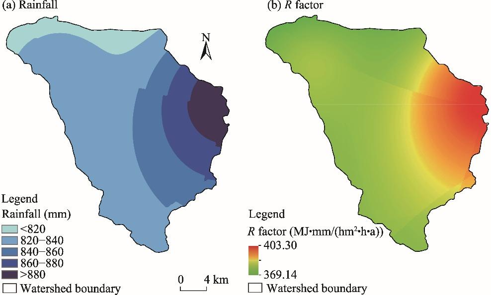
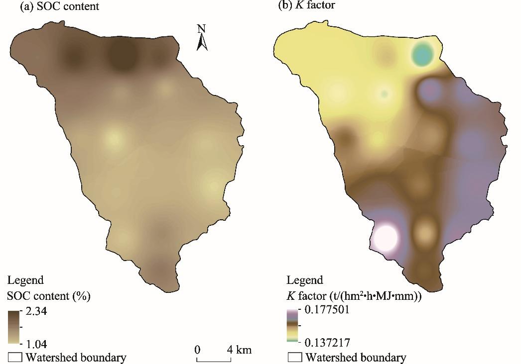
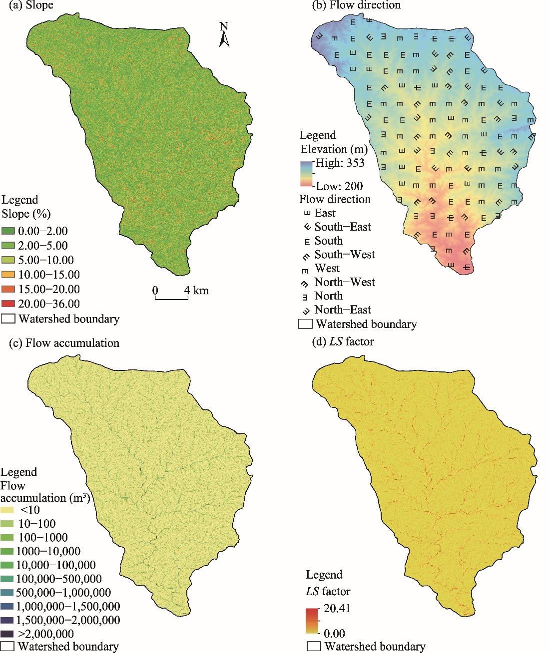
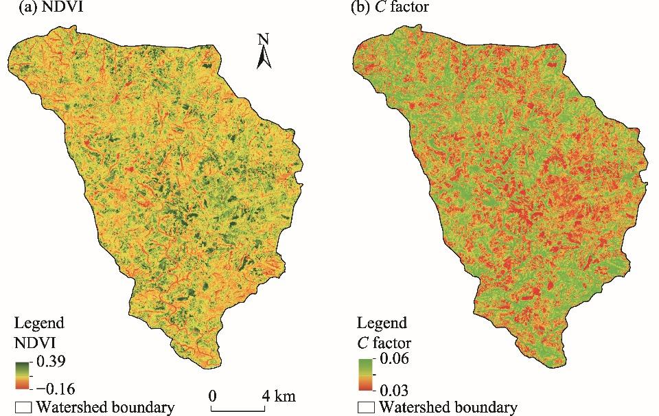
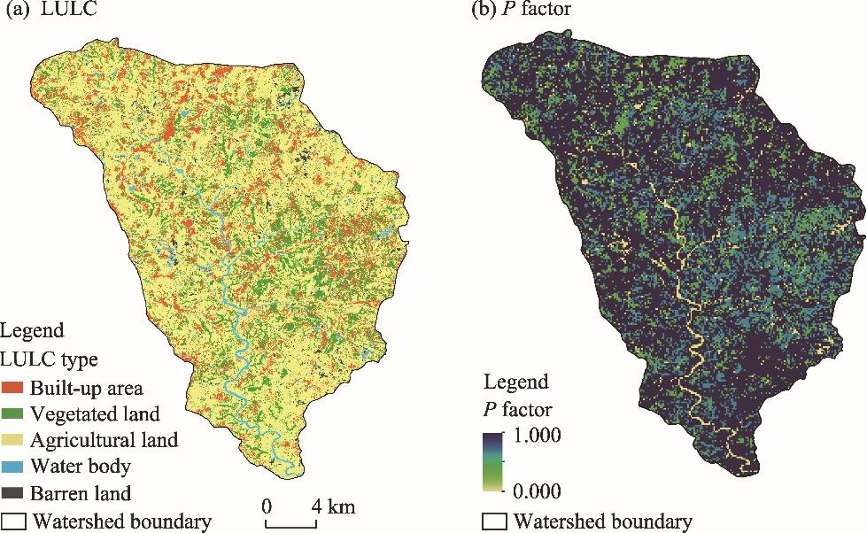
Human activities to improve the quality of life have accelerated the natural rate of soil erosion. In turn, these natural disasters have taken a great impact on humans. Human activities, particularly the conversion of vegetated land into agricultural land and built-up area, stand out as primary contributors to soil erosion. The present study investigated the risk of soil erosion in the Irga watershed located on the eastern fringe of the Chota Nagpur Plateau in Jharkhand, India, which is dominated by sandy loam and sandy clay loam soil with low soil organic carbon (SOC) content. The study used the Revised Universal Soil Loss Equation (RUSLE) and Geographical Information System (GIS) technique to determine the rate of soil erosion. The five parameters (rainfall-runoff erosivity (R) factor, soil erodibility (K) factor, slope length and steepness (LS) factor, cover-management (C) factor, and support practice (P) factor) of the RUSLE were applied to present a more accurate distribution characteristic of soil erosion in the Irga watershed. The result shows that the R factor is positively correlated with rainfall and follows the same distribution pattern as the rainfall. The K factor values in the northern part of the study area are relatively low, while they are relatively high in the southern part. The mean value of the LS factor is 2.74, which is low due to the flat terrain of the Irga watershed. There is a negative linear correlation between Normalized Difference Vegetation Index (NDVI) and the C factor, and the high values of the C factor are observed in places with low NDVI. The mean value of the P factor is 0.210, with a range from 0.000 to 1.000. After calculating all parameters, we obtained the average soil erosion rate of 1.43 t/(hm2•a), with the highest rate reaching as high as 32.71 t/(hm2•a). Therefore, the study area faces a low risk of soil erosion. However, preventative measures are essential to avoid future damage to productive and constructive activities caused by soil erosion. This study also identifies the spatial distribution of soil erosion rate, which will help policy-makers to implement targeted soil erosion control measures.

Cite this article

Ratan PAL , Buddhadev HEMBRAM , Narayan Chandra JANA . Assessment of soil erosion in the Irga watershed on the eastern edge of the Chota Nagpur Plateau, India[J]. Regional Sustainability, 2024 , 5(1) : 100112 . DOI: 10.1016/j.regsus.2024.03.006

1. Introduction

Soil erosion is a naturally occurring geomorphic process called geological erosion, which occurs at a rate almost equal to that of soil formation (Smoot and Smith, 1999). However, soil erosion is no longer solely a natural process and has become more and more serious as a result of human activities, such as the pursuit of increased profits (FAO, 2019). The rate of soil erosion is positively correlated with the intensity of human activities (Leh et al., 2011; Wu and Xie, 2011; Ding et al., 2015), and poor land management is probably the most active controlling factor of soil erosion (Nadeu et al., 2012; Montgomery et al., 2014; Niu et al., 2015; Liu, 2016; Issaka and Ashraf, 2017). A study conducted by Don and Leet (1965) estimated that the amount of sediment carried by rivers increased from 9.90×10⁶ t/a before plant domestication to 26.50×10⁶ t/a in the 1960s. Globallyabout 75.00×10⁶ t of soil is eroded from the land every year, with the rate about 13-40 times faster than the natural erosion rate (Zuazo et al., 2009; Rahaman et al., 2015). Soil erosion rate is particularly high in Asia, Africa, and South America, averaging 30-40.00 t/(hm2•a) (Pimentel, 2006; Moncef et al., 2011; Shit et al., 2015). The Asian region experiences the highest rate of soil erosion, at 40.00 t/(hm2•a) (El-Swaify, 1997; Rahaman et al., 2015). According to the estimation by Ayoub et al. (1991), the area of soil erosion accounts for about 84.00% of the total global area under soil degradation. It is estimated that the total land area of soil degradation affected by human activities is 2.00×10⁶ hm2 of the total soil degradation area subjected to human-induced soil degradation. Oldeman (1992) utilized the Global Assessment of Soil Degradation (GLASOD) data to determine the land area under soil degradation at global scale, estimating that about 1.10×10⁶ and 0.50×10⁶ hm2 of land is affected by water and wind erosion, respectively (Biggelaar et al., 2003). Some researchers (Brown and Wolf, 1984; Lal, 1994; Eaton, 1996; Biggelaar et al., 2003) expressed concerns that if the present rate of soil erosion continues without proper land management practices, a considerable proportion of productive land may lose its economic or biological importance.
In India, about 53.00% of the total land area (1.75×10⁸ hm2 out of 3.28×10⁸ hm2) suffers from soil erosion (Narayan and Babu, 1983). Soil erosion is particularly severe in the Himalayan regions, northern and eastern states of India, and Western Ghats (India). These regions together constitute about 45.00% of the total erosion-prone area in India, and are affected by factors such as gullies, ravines, sheet flows, shifting cultivation, irrigation, grazing, and waterlogging (Narayan and Babu, 1983; Singh et al., 1992; Pandey et al., 2007; Rahaman et al., 2015). The land influenced by soil erosion accounts for about 87.00% of the total degraded land in India (UNEP, 2001). The average annual rate of soil erosion is 16.35 t/(hm2•a) in India, equivalent to 5.30×10⁶ t of soil eroded each year. Of this, about 29.00% of eroded soil is deposited in seas, 10.00% in reservoirs, and the remaining 61.00% is displaced across different locations (Narayan and Babu, 1983).
The National Bureau of Soil Survey and Land Use Planning (NBSS & LUP, 2014) collaborated to assess the status of soil erosion in state of Jharkhand, India. Their investigation revealed that about 35.00% of the total land in Jharkhand is minimally impacted by soil erosion and can be easily managed. Another 27.00% of the total land is moderately affected, while the remaining 38.00% is severely affected and needs intensive care. Land use and land cover (LULC) changes and mining activities are regarded as the major causes of soil erosion in Jharkhand (Mhaske et al., 2021).
Concerns have been raised about Jharkhand, as about 65.00% of its land is prone to moderate and high levels of soil erosion. This is alarming, as it could increase soil erosion rate and the area of high erosion rate, exerting negative impacts on crop yield, gross agricultural production, and ultimately, food security. Hence, it is crucial to understand the current rate of soil erosion as a form of land degradation, especially in areas dominated by agricultural and mining activities. The present study seeks to identify the intensity, spatial distribution, and nature of soil erosion, and the main factors causing soil erosion in the Irga watershed located on the eastern fringe of the Chota Nagpur Plateau in Jharkhand, India. These initial steps are crucial for resolving this serious issue. This study can be valuable for land use planners in effectively managing and utilizing land and may inspire further research to develop effective strategies for reducing soil erosion rate in this region.

2. Materials and methods

2.1. Study area

According to the micro-watershed atlas of Jharkhand (Soil and Land Use Survey of India, 2017), the Irga watershed (24°10°07′′N-24°30°12′′N, 85°10°26′′E-86°50°34′′E) is a sub-watershed of No. 2A2I6 (https://slusi.dacnet.nic.in/dmwai/JHARKHAND/Districts/GIRIDIH.html). The watershed is located on the eastern edge of the Chota Nagpur Plateau and falls within the jurisdiction of Giridih District in Jharkhand. The study area covers a total area of 4.80×10⁵ hm2. The climate of the study area can be characterized as the tropical sub-humid dry bioclimatic type (Velayutham et al., 1999). The monsoon is the predominant factor influencing rainfall, with about 80.00% of the total annual rainfall occurring during the rainy season (June-September). The average annual rainfall is reported to be 840.000 mm and the annual average temperature is 25°C (Roy, 2019), ranging from 10°C to 47°C (Kumar et al., 2016). The study area lies over the Koderma Plateau, which is a part of the Eastern Plateau in India (Velayutham et al., 1999; Roy, 2019). The Irga River is one of the major left-hand tributaries of the Barakar River (Fig. 1). The north of the watershed is surrounded by the Gangetic Plain of South Bihar, the Ushree River Basin to the east, and the Barakar River to the south. A total of 19 soil sampling sites were designed in the field (Fig. 1).
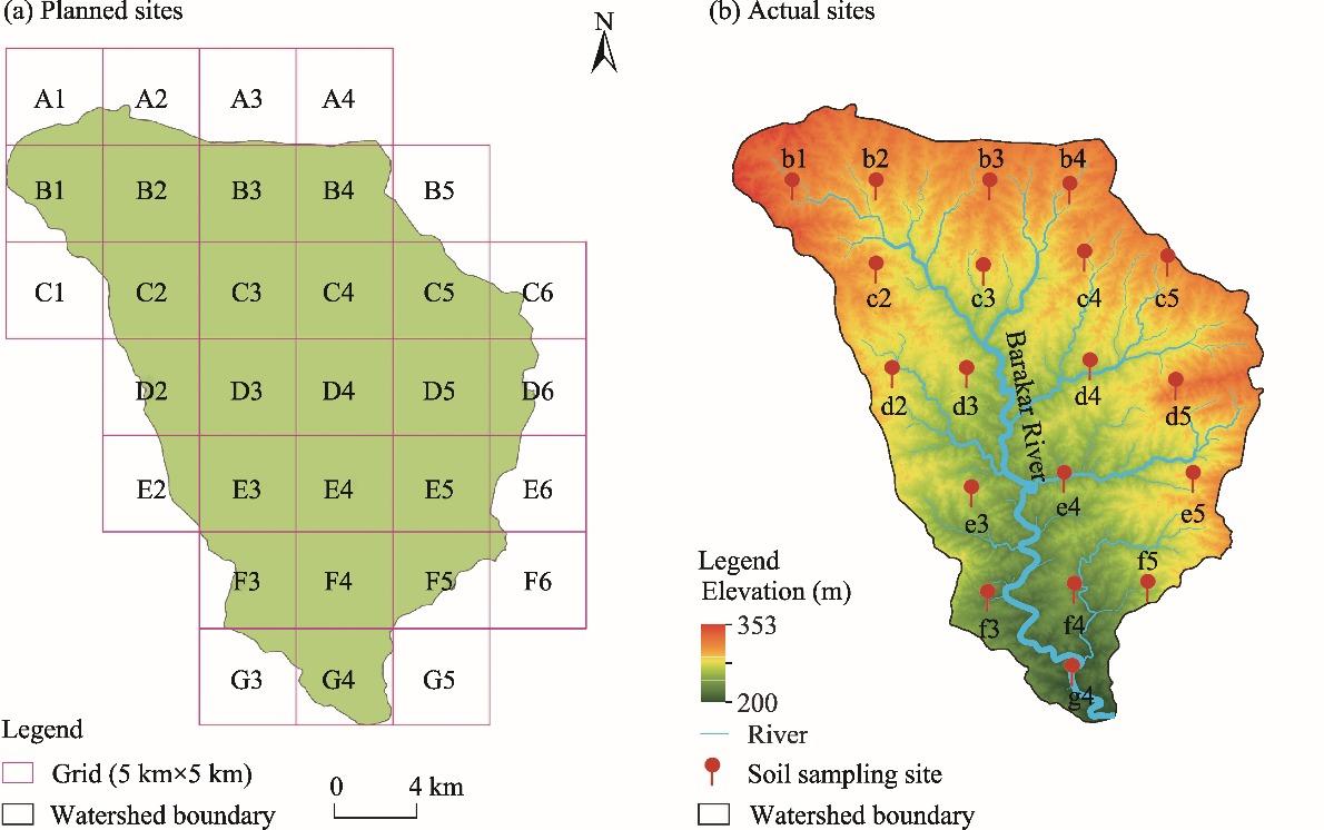
Fig. 1. Planned (a) and actual (b) sites of soil sample collection in the study area.

2.2. Data sources

Four topographical maps (G45T15, G45T16, G45U3, and G45U4) at a scale of 1:50,000 were collected from the Survey of India (http://soinakshe.uk.gov.in). Google Earth (https://www.google.cn/intl/zh-en/earth/) was frequently used to obtain and verify topographical information. A map of digital elevation model (DEM) with a resolution of 12.5 m was downloaded from the Alaska Satellite Facility (https://www.afs.alaska.edu). Furthermore, monthly average rainfall data in 2009-2019 were collected from the Indian Meteorological Department. A satellite image (Landsat 8; acquisition date: 31 January 2020; Path/Row: 140/43) was used for calculating Normalized Difference Vegetation Index (NDVI) and generating LULC map (Fig. 2).
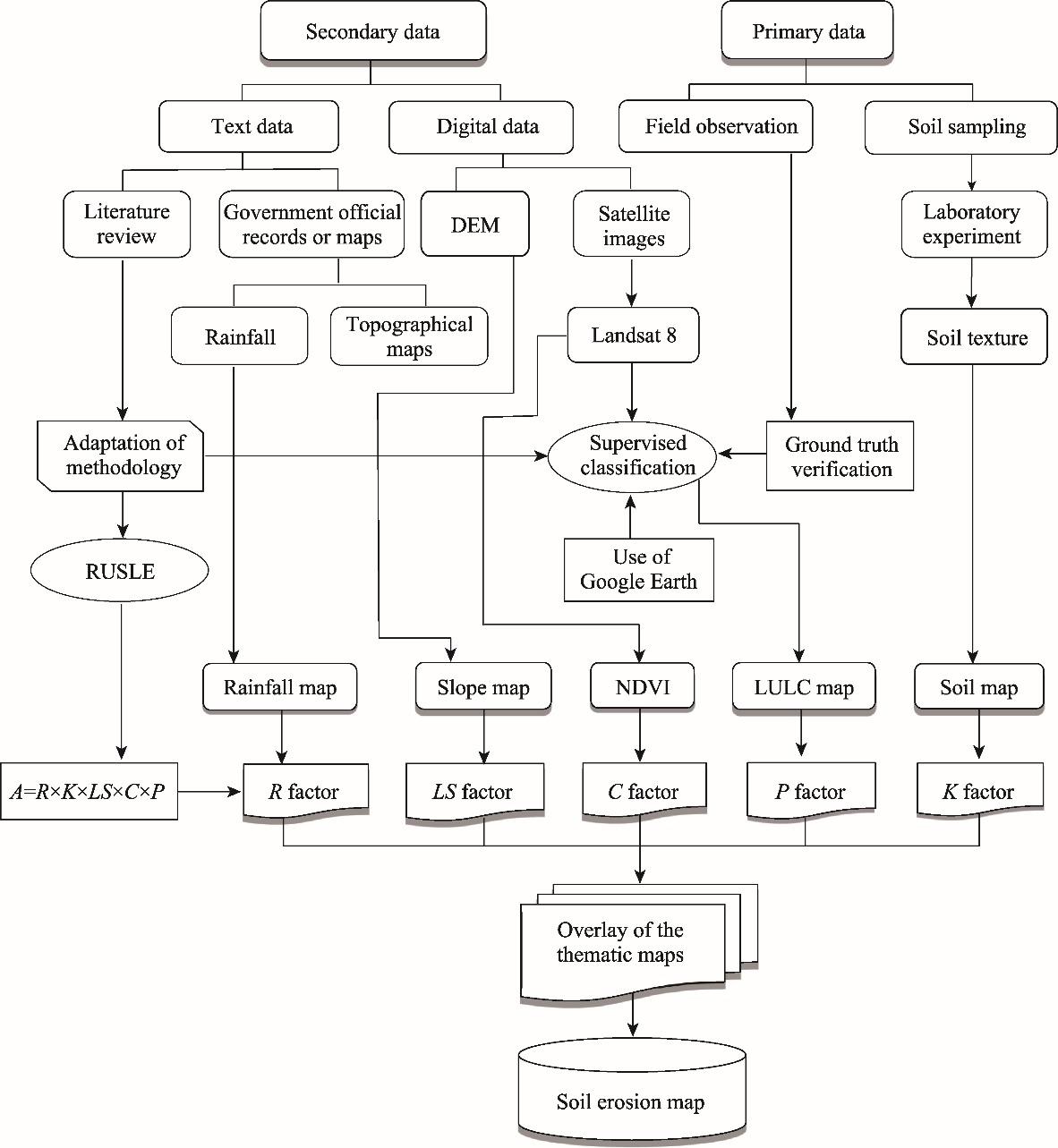
Fig. 2. Methodological flow chart of this study. DEM, digital elevation model; NDVI, Normalized Difference Vegetation Index; LULC, land use and land cover; RUSLE, Revised Universal Soil Loss Equation; A, average annual rate of soil erosion; R, rainfall-runoff erosivity; LS, slope length and steepness; C, cover-management; P, support practice; K, soil erodibility.
Soil samples were collected in January 2021 using the systematic random sampling method during a field survey and were subsequently analyzed in the laboratory. Specifically, to collect soil samples, we divided the study area into several equal-sized grids (2.50×10³ hm2 for each), each of which collected one sample. Soil samples were primarily collected from the middle of each grid, excluding grids whose centers were not in the study area. Subsequently, each soil sample was examined in the laboratory to determine soil texture and soil organic carbon (SOC) content. The sieving method was used to determine soil texture, involving drying at room temperature and the breakdown of soil samples. Materials with particle size larger than 2.000 mm in diameter, such as stones, gravels, and pebbles, were removed through sieving with a 2.000 mm sieve. Following this, 250.00 g of soil sample was sieved again to determine soil texture, following the suggestions from the United States Department of Agriculture (USDA) (Rebecca, 2009). After sieving, the soil in each diameter group was weighted to determine the contents of sand, silt, and clay. The titration method of Walkley and Black (1934) was used to determine SOC:
$ \mathrm{SOC}=\frac{V(B-T)}{B} \times \frac{0.3}{W} \times \frac{100+m}{100} \times \mathrm{RF},$
where SOC is the soil organic carbon (%); V is the volume of 0.167 mol/L K2Cr2O7 solution (mL); B and T are the volumes (mL) of ferrous ammonium sulfate reagent for blank and soil sample, respectively; W is the weight of soil sample (g); m is the air-dry moisture percentage of the soil sample used (%); and RF is the recovery factor (1.30). In the determination of SOC, the correction factor was set as 1.30 (recovery of 77.00%) (Bhattacharyya et al., 2015). The content of SOC was determined using the titration method of Walkley and Black (1934).

2.3. Data processing

The Revised Universal Soil Loss Equation (RUSLE) (Renard et al., 1997), an enhanced version of the universal soil loss equation (Wischmeier and Smith, 1965), is one of the most widely used models to estimate the average annual rate of soil erosion. The model was originally developed from extensive data collected over several years from 1.00×10⁴ small test plots in the United States, and its application in tropical areas may not yield as satisfactory results as observed in temperate zones. Therefore, many researchers have tried to increase the applicability of the model in tropical regions through optimization. In the present study, such optimization was adopted while preserving the basic format of the model. The adopted model provides satisfactory results in tropical regions, rendering it a suitable choice for the present study.
The RUSEL was designed by multiplying the effects of the five most important factors influencing soil erosion (Renard et al., 1997).
$ A=R \times K \times L S \times C \times P \text {, }$
where A is the average annual rate of soil erosion (t/(hm2•a); R is the rainfall-runoff erosivity (MJ•mm/(hm2•h•a)); K is the soil erodibility (t/(hm2•h•MJ•mm)); LS is the slope length and steepness; C is the cover-management; and P is the support practice.

2.3.1. Rainfall-runoff erosivity (R) factor

The R factor is the rainfall erosion index plus an additional factor for any significant runoff from snowmelt. When calculating the R factor, it is considered that factors other than R factor remain constant, and soil erosion is directly proportional to the rainstorm parameters (Renard et al., 1997). The value of the R factor (seasonal and annual scales) was calculated using the average annual rainfall data. The geo-environmental condition of India is distinct compared with the United States; hence, it is important to revise the equation to adapt to Indian conditions. Babu et al. (1978) revised correlation between average annual rainfall and average seasonal rainfall and proposed an average annual erosion index applicable to Indian conditions.
$ R_{a}=79+0.363 P_{a},$
$ R_{S}=50+0.389 P_{S} \text {, }$
where Ra is the average annual erosion index (MJ•mm/(hm2•h•a)); Pa is the average annual rainfall (mm); Rs is the seasonal erosion index (MJ•mm/(hm2•h•a)); and Ps is the average seasonal rainfall (mm).

2.3.2. Soil erodibility (K) factor

The soil property method was used to calculate the K factor. In this method, soil properties, such as the percentages of silt, sand, and clay, and the content of SOC, were determined in the laboratory. The following equations were used to determine the K factor (Williams, 1995):
$ K=f_{\text {csand }} \times f_{\text {cl-si }} \times f_{\text {orgc }} \times f_{\text {hisand }},$
$ f_{\text {csand }}=0.2+0.3 \times \exp ^{-0.256 \times m_{s}\left(1-\frac{m_{\text {silt }}}{100}\right)} \text {, }$
$ f_{\mathrm{cl}-\mathrm{si}}=\left(\frac{m_{\mathrm{silt}}}{m_{c}+m_{\mathrm{silt}}}\right)^{0.3},$
$ f_{\text {orgc }}=1-0.25 \times \mathrm{SOC}+\exp ^{3.72-2.95 \times \text { orgc }},$
$ f_{\text {hisand }}=1-\frac{0.7 \times \frac{1-m_{\mathrm{s}}}{100}}{\frac{1-m_{\mathrm{s}}}{100}}+\exp ^{-5.51+22.9 \times\left(\frac{1-m_{\mathrm{s}}}{100}\right)}$
where fcsand is the factor that assigns low K factor for soils with high coarse sand content and high K factor for soils with low sand content; fcl-si is the factor that distributes low K factor value for soils with high clay to silt ratio; forgc is the factor that reduces K factor for soils with high organic carbon content; fhisand is the factor that decreases K factor for soils with extremely high sand content; ms is the percentage of sand (%); msilt is the percentage of silt (%); and mc is the percentage of clay (%).

2.3.3. Slope length and steepness (LS) factor

Digital elevation model (DEM) was used to extract information regarding the slope of the Earth’s surface. In the present study, the LS factor was considered as a single parameter, which was determined using the following equation (Moore and Burch, 1985):
$ L S=\left(\frac{A_{s}}{22.13}\right)^{k} \times\left(\frac{\sin \theta}{0.0896}\right)^{n},$
where As is the specific catchment area (m2); k varies from 0.4 to 0.6; θ is the gradient of slope in degree (°); and n ranges from 1.2 to 1.3.

2.3.4. Cover-management (C) factor

The NDVI was used to determine the C factor, following the recommendation of van der Knijff et al. (2000) under the European conditions. Durigon et al. (2014) reported that the estimation of the C factor in tropical climatic regions using the equation suggested by van der Knijff et al. (2000) tends to be high because of the increased rainfall intensity. Therefore, they modified the equation. The formula was again modified by Colman et al. (2018) after comparing the computed values with experimental field data. Then, their results (Colman et al., 2018) showed that the method developed by Durigon et al. (2014) suffered from tenfold systematic biases, so a correction was introduced using 0.1 as an input (Almagro et al., 2019).
$ C_{r A}=\frac{-\mathrm{NDVI}+1}{2} \times 0.1,$
where CrA is the estimated C factor.

2.3.5. Support practice (P) factor

In the study area, the local population does not engage in any soil conservation practices, but their activities, specifically farming, contribute to soil erosion. Consequently, the P factor value is not fixed at 1.000 but is determined using the LULC map. We assigned the P factor value (see Table 1) for each LULC type is assigned according to the guidelines provided by the United States Department of Agriculture-Soil Conversion Service (USDA-SCS, 1972).
Table 1 Support practice (P) factor for different land use and land cover (LULC) types.
LULC type P factor value LULC type P factor value
Built-up area 0.002 Water body 0.000
Agricultural land 0.280 Barren land 1.000
Vegetated land 0.005

3. Results and discussion

3.1. Estimation of input parameters of the Revised Universal Soil Loss Equation (RUSLE)

3.1.1. Spatial distribution characteristics of the R factor

Based on the historical monthly rainfall data recorded from 2009 to 2019, this study used inverse distance weighting method to calculate average annual rainfall (Fig. 3a), which ranges from 799.270 to 893.380 mm, with mean and standard deviation values of 840.000 and 20.300 mm, respectively. The eastern part of the Irga watershed receives the highest rainfall, gradually decreasing towards other parts (Fig. 3a).
Fig. 3. Spatial distribution of average annual rainfall (a) and R factor (b).
As the R factor is positively correlated with rainfall, it follows the same distribution pattern as the rainfall (Fig. 3). The R factor varies from 369.14 to 403.30 MJ•mm/(hm2•h•a), with mean and standard deviation values of 383.92 and 7.27 MJ•mm/(hm2•h•a), respectively.
In the Irga watershed, two different distribution patterns of rainfall are observed in the four seasons (as classified by the Indian Metrological Department), including winter (December-February of the next year), pre-monsoon season (March-May), monsoon season (June-September), and post-monsoon season (October-November) (Fig. 4a-d). During winter and monsoon season, the northwestern region is characterized by the highest rainfall, gradually decreasing towards the southeast (Fig. 4a and c). Conversely, during pre-monsoon and post-monsoon seasons, the highest rainfall is found in the eastern part, decreasing from east to northwest (Fig. 4b and d).
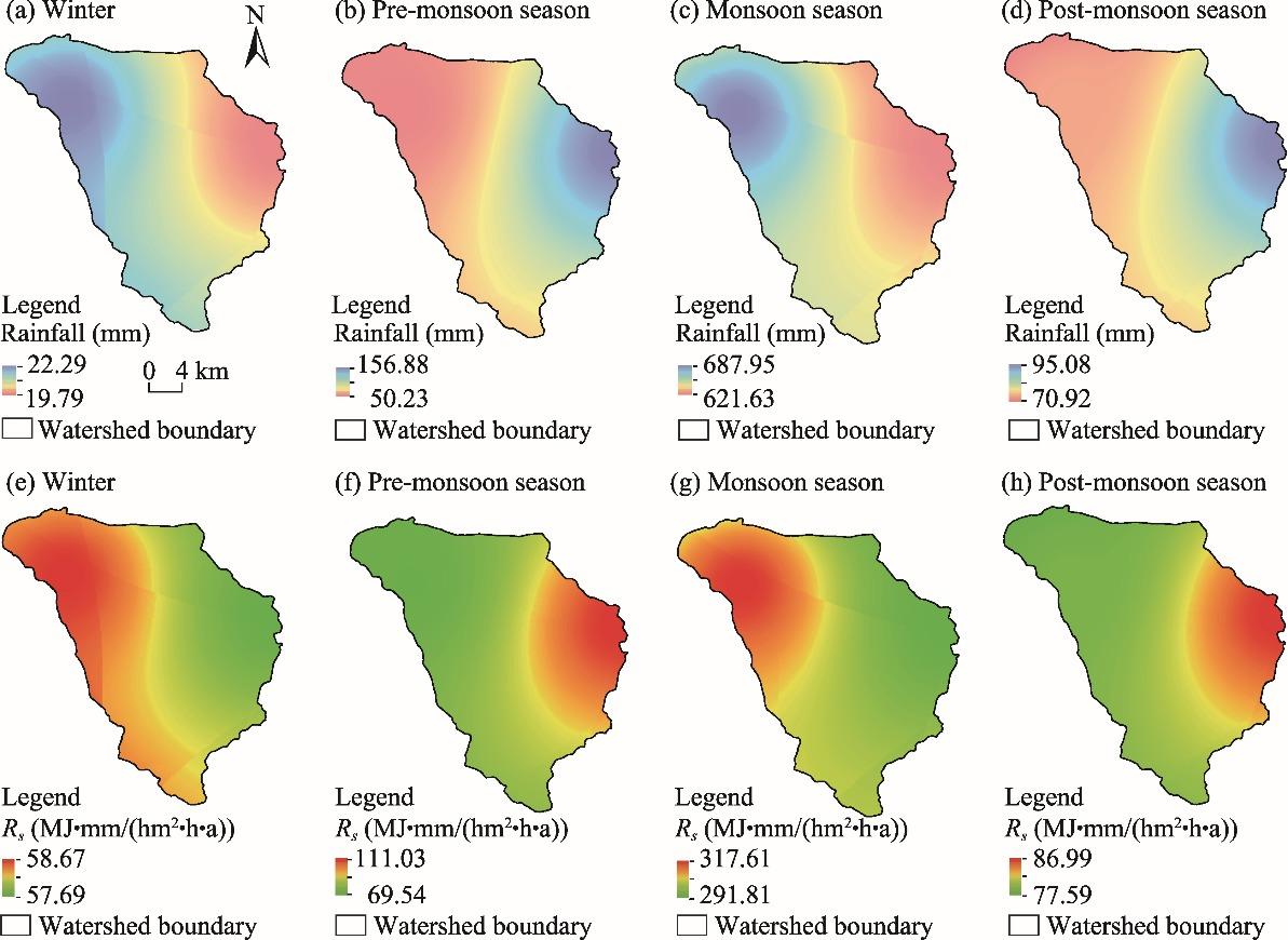
Fig. 4. Spatial distribution of rainfall in winter (a), pre-monsoon season (b), monsoon season (c), and post-monsoon season (d), as well as spatial distribution of seasonal erosion index (Rs) in winter (e), pre-monsoon season (f), monsoon season (g), and post-monsoon season (h).
Alongside the R factor, the Rs was also calculated to understand erosion periods properly and develop appropriate erosion control strategies (Fig. 4e-h). The Rs for four seasons was calculated using seasonal rainfall data. From Figure 4 we can see that the distribution pattern of Rs is the same as that of rainfall in the study area.

3.1.2. Spatial distribution characteristics of the K factor

The percentage of sand in the soil varies from 35.64% (soil sample c3) to 71.71% (f4), corresponding to 15.50% (f4) to 34.61% (c5) for slit, and 12.79% (f4) to 42.02% (c3) for clay (Fig. 5). Notably, for soil sample f4, the content of sand is the highest, while the contents of silt and clay are the lowest. The southern part of the study area is characterized by higher contents of sand (Fig. 5a) and silt (Fig. 5b), whereas clay has a higher content in the north (Fig. 5c). Furthermore, the diameters of clay, silt, and sand are considered as <0.002, 0.002-0.050, and 0.050-2.000 mm, respectively, following the guideline of United States Department of Agriculture-Natural Resources Conservation Service (USDA-NRCS, 2000). Five major soil texture categories were identified by using the textural triangle of the United States Department of Agriculture (USDA). Sandy clay loam and clay occupy the northern part of the Irga watershed. The middle part is dominated by sandy loam and loam, while the southern part is leaded by sandy loam and sandy clay loam (Fig. 5d; Table 2).
Fig. 5. Spatial distribution of sand (a), silt (b), clay (c), and soil texture (d).
Table 2 Description of the collected 19 soil samples.
Soil sample Latitude (N) Longitude (E) Weight of sand (g) Weight of silt (g) Weight of clay (g) Percentage of sand (%) Percentage of silt (%) Percentage of clay (%) Soil texture
b1 24°25′57′′ 85°54′48′′ 139.72 44.17 66.11 55.89 17.67 26.44 Sandy clay loam
b2 24°25′57′′ 85°57′23′′ 124.11 50.73 75.16 49.64 20.29 30.06 Sandy clay loam
b3 24°25′58′′ 86°00′49′′ 133.01 51.02 65.97 53.20 20.41 26.39 Sandy clay loam
b4 24°25′59′′ 86°03′17′′ 103.68 45.15 101.17 41.47 18.06 40.47 Clay
c2 24°23′38′′ 85°57′24′′ 118.59 47.87 83.54 47.44 19.15 33.42 Sandy clay loam
c3 24°23′37′′ 86°00′39′′ 89.10 55.86 105.04 35.64 22.34 42.02 Clay
c4 24°23′57′′ 86°03′46′′ 145.18 61.09 43.73 58.07 24.44 17.49 Sandy loam
c5 24°23′55′′ 86°06′22′′ 112.55 75.87 61.58 45.02 30.35 24.63 Loam
d2 24°20′43′′ 85°57′56′′ 163.65 43.55 42.8 65.46 17.42 17.12 Sandy loam
d3 24°20′45′′ 86°00′11′′ 104.74 57.01 88.25 41.90 22.80 35.30 Clay loam
d4 24°20′56′′ 86°03′57′′ 136.96 50.79 62.25 54.78 20.32 24.90 Sandy clay loam
d5 24°20′25′′ 86°06′35′′ 131.61 63.92 54.47 52.64 25.57 21.79 Sandy clay loam
e3 24°17′21′′ 86°00′20′′ 101.42 73.46 75.12 40.57 29.38 30.05 Clay loam
e4 24°17′49′′ 86°03′10′′ 106.38 65.76 77.86 42.55 26.30 31.14 Clay loam
e5 24°17′ 46′′ 86°07′10′′ 116.59 73.24 60.17 46.64 29.30 24.07 Loam
f3 24°14′27′′ 86°00′54′′ 126.30 86.53 37.17 50.52 34.61 14.87 Loam
f4 24°14′42′′ 86°03′33′′ 179.27 38.76 31.97 71.71 15.50 12.79 Sandy loam
f5 24°14′22′′ 86°05′48′′ 134.86 66.97 48.17 53.94 26.79 19.27 Sandy loam
g4 24°12′22′′ 86°03′30′′ 114.75 65.67 69.58 45.90 26.27 27.83 Sandy clay loam
The average content of SOC is 1.44% in the Irga watershed, and the content varies from 1.04% (d3) to 2.34% (b3) (Table 3). The highest content of SOC is observed in the northern part, while the lowest is in the middle, and there is a moderate content of SOC in the south of the study area (Fig. 6a). The K factor varies from 0.137217 to 0.177501 t/(hm2•h•MJ•mm), with mean and standard deviation values of 0.156000 and 0.007000 t/(hm2•h•MJ•mm), respectively. The study area can be divided into two unequal parts, with low K factor values in the northern part and comparatively high K factor values in the southern part (Table 3; Fig. 6b).
Table 3 Soil erodibility (K) factor and soil organic carbon (SOC) of the collected 19 soil samples.
Soil sample fcsand fcl−si forgc fhisand K factor
(t/(hm2•h•MJ•mm))
SOC content (%)
b1 0.200002 0.759957 0.978409 0.996884 0.148248 1.66
b2 0.200012 0.761346 0.975602 0.999146 0.148436 2.04
b3 0.200006 0.77961 0.974846 0.998209 0.151732 2.34
b4 0.200050 0.702759 0.976176 0.999847 0.137217 1.92
c2 0.200016 0.738636 0.978914 0.999462 0.144546 1.62
c3 0.200251 0.728054 0.983048 0.999956 0.143316 1.38
c4 0.200004 0.850468 0.985746 0.995129 0.166856 1.26
c5 0.200098 0.836715 0.982229 0.999676 0.164396 1.42
d2 0.200000 0.814362 0.985746 0.978726 0.157136 1.26
d3 0.200076 0.755338 0.991004 0.999833 0.149740 1.04
d4 0.200004 0.786618 0.985276 0.997517 0.154626 1.28
d5 0.200013 0.831183 0.988640 0.998405 0.164097 1.14
e3 0.200196 0.809519 0.987670 0.999873 0.160044 1.18
e4 0.200098 0.791087 0.986702 0.999808 0.156160 1.22
e5 0.200065 0.835349 0.990543 0.999545 0.165468 1.06
f3 0.200064 0.898337 0.988640 0.998975 0.177501 1.14
f4 0.200000 0.834899 0.981460 0.932127 0.152761 1.46
f5 0.200012 0.849956 0.985276 0.997913 0.167149 1.28
g4 0.200052 0.805135 0.978914 0.999610 0.157611 1.62

Note: where fcsand is the factor that assigns low K factor for soils with high coarse sand content and high K factor for soils with low sand content; fcl-si is the factor that distributes low K factor value for soils with high clay to silt ratio; forgc is the factor that reduces K factor for soils with high organic carbon content; fhisand is the factor that decreases K factor for soils with extremely high sand content.

Fig. 6. Spatial distribution of soil organic carbon (SOC) content (a) and the K factor (b).

3.1.3. Spatial distribution characteristics of the LS factor

DEM was used to prepare the slope map (in percentage) (Fig. 7a), which indicates that the study area is considerably flat. The mean and standard deviation values of slope in the study area are 4.94% and 3.09%, respectively (Table 4). Approximately 70.11% (3.36×10⁴ hm2) of the total area is below 5.00% of the slope, while only 2.00% of the area (957.00 hm2) has a slope more than 15.00%. The areas with slopes of 5.00%-10.00% and 10.00%-15.00% are 21.50% (1.03×10⁴ hm2) and 6.39% (0.31×10⁴ hm2), respectively (Table 4). The direction of water flow was determined by the slope direction, as depicted by arrows in Figure 7b. Additionally, a flow accumulation map (Fig. 7c) was used to understand surface runoff accumulated into a specific grid. The higher surface runoff accumulated into a specific grid, the higher the amount of water flowing off that grid. In other words, flow accumulation determines the area that contributes to each cell upstream. The value of flow accumulation increases with increasing runoff, hence a high flow accumulation value indicates stream or river. The LS factor value ranges from 0.00 to 20.41, with a mean value of 2.74 (Fig. 7d). The low mean value of the LS factor is attributed to the flat terrain, with a limited elevation of 153 m. Riverbank areas exhibit a considerably high LS factor value, indicating potential concerns about riverbank erosion in the study area. Notably, the RUSLE model does not consider whether the slope is concave, convex, or mixed (Oliveira et al., 2013).
Fig. 7. Spatial distribution of slope (a), flow direction (b), flow accumulation (c), and the LS factor (d).
Table 4 Area and percentage of slope in the Irga watershed.
Slope (%) Area (104 hm2) Area percentage (%) Mean slope (%) Standard deviation (%)
0.00-2.00 0.84 17.53 4.94 3.09
2.00-5.00 2.52 52.58
5.00-10.00 1.03 21.50
10.00-15.00 0.31 6.39
15.00-20.00 0.07 1.53
20.00-36.00 0.02 0.47

3.1.4. Spatial distribution characteristics of the C factor

The present study used NDVI to determine the C factor; NDVI is one of several indices commonly applied in research to highlight vegetation-covered areas using remote sensing data (Bhandari et al., 2012). NDVI quantifies vegetation by using the reflectance of the red (600-700 nm) and near-infrared (750-1300 nm) bands from vegetation (Nageswara et al., 2005). The NDVI follows the principle that vegetation (green leaves) absorbs red band and reflects near-infrared band. The NDVI values vary from −1.00 to 1.00, where higher values indicate denser vegetation cover, and vice versa (Almagro et al., 2019). Negative NDVI values generally represent water, snow, sand, or clouds, while NDVI values close to 0.00 indicate bare soil and rocks, and meadows and shrubs are represented by NDVI values of 0.20−0.30 (Hu et al., 2008; Xie et al., 2010; Achibeta et al., 2014; Deep and Saklani, 2014; Gandhi et al., 2015).
In the present study, NDVI values vary from −0.16 to 0.39, with mean and standard deviation values of 0.17 and 0.04, respectively (Fig. 8a). The central and east-central regions of the study area show the highest NDVI values, while rivers and water bodies have negative NDVI values. Owing to the negative linear correlation between NDVI and the C factor, the high C factor values are observed in places with low NDVI values. The C factor values range from 0.03 to 0.06, with a mean of 0.04 (Fig. 8b).
Fig. 8. Spatial distribution of NDVI (a) and the C factor (b).

3.1.5. Spatial distribution characteristics of the P factor

The people of the study area, especially farmers, demonstrated limited concern for soil erosion and its conservation. Farmers have not undertaken specific activities to mitigate soil erosion although occasional practices such as strip cropping, contour plowing, and crop rotation were observed during field observations. Notably, these practices are primarily driven by farmers’ intention to enhance production rather than a focused effort to conserve soil. Considering all these observations, the P factor values for each LULC type have been assigned, adopting values from USDA-SCS (1972). Subsequently, this study obtains the spatial distribution of LULC and the P factor (Fig. 9).
Fig. 9. Spatial distribution of LULC (a) and the P factor (b).

3.2. Estimation of soil erosion

The RUSLE was used to estimate the soil erosion rate in the Irga watershed, and all the required parameters were determined through standardized methods. The R factor for the study area was calculated using average annual rainfall data, exhibiting a range from 369.14 to 403.30 MJ•mm/(hm2•h•a), with a mean value of 383.92 MJ•mm/(hm2•h•a). For a comprehensive understanding of the high and low erosivity, the Rs was calculated for all four seasons. By the study of the Rs, two completely different situations are observed. In winter and monsoon season, the highest Rs is observed in the northwestern part, contrasting with pre-monsoon and post-monsoon seasons where the lowest Rs value is found. The K factor ranges from 0.137217 to 0.177501 t/(hm2•h•MJ•mm), with a mean value of 0.156000 t/(hm2•h•MJ•mm). Five soil texture categories are found in the study area: sandy clay loam, sandy loam, loam, clay, and clay loam. The soil is dominated by a high percentage of sand, while SOC shows a low content ranging from 1.04% to 2.34% (with an average of 1.44%). The computation of the K factor is based on soil texture and SOC (Table 3). The LS factor was calculated from DEM, varing from 0.00 to 20.41 (with a mean value of 2.74). The slope of the Irga watershed is considerably flat, ranging from 0.00% to 36.00% with a mean slope of 4.94%. This signifies a less impact of the LS factor on soil erosion. For the determination of the C factor, the NDVI map was used. The C factor ranges from 0.03 to 0.06, with an average of 0.04. There are no considerable practices dedicated to protect against soil erosion. The mean value of the P factor is 0.210, within a range from 0.000 to 1.000. After calculating all parameters, they were multiplied through the raster calculator in ArcGIS to obtain the soil erosion map (Fig. 10).
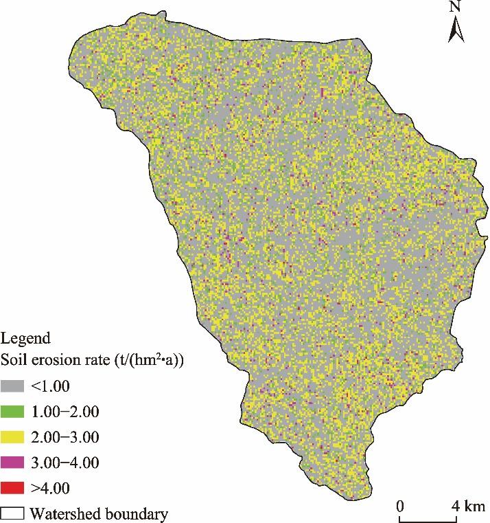
Fig. 10. Spatial distribution of soil erosion rate in the Irga watershed.
The soil erosion rate within the study area ranges from 0.00 to 32.71 t/(hm2•a), with a mean rate of 1.43 t/(hm2•a). In the year 2020, about 6.90×10⁴ t of soil was eroded from the watershed. The distribution of soil erosion rate exhibits a remarkably uniform pattern across the study area, with an absence of specific zones characterized by extremely high or low soil erosion rate (Fig. 10). Notably, this study assigned the risk categories based on the observed soil erosion rate in the study area. Approximately half of the Irga watershed (50.41% of the study area) exhibits a mean soil erosion rate of <1.00 t/(hm2•a), categorized as a very low risk level (Table 5). The area with low risk category covers about 7.95% (0.38×10⁴ hm2) of the study area, while the area with moderate risk category encompasses about 34.28% (1.64×10⁴ hm2). A very small area falls under the high risk (5.32%) and very high risk (2.04%) categories (Table 5).
Table 5 Soil erosion rate under different risk categories in the Irga watershed.
Soil erosion rate (t/(hm2•a)) Risk category Area (104 hm2) Area percentage (%)
<1.00 Very low 2.42 50.41
1.00−2.00 Low 0.38 7.95
2.00−3.00 Moderate 1.64 34.28
3.00−4.00 High 0.26 5.32
>4.00 Very high 0.10 2.04

4. Conclusions

Soil erosion is a natural phenomenon observed in various places around the world. Unfortunately, it has become a crucial concern owing to improper land management, emerging as a major global issue requiring attention.
Among the various causes of soil erosion, anthropogenic causes are the dominant controlling factors, which lead to especially changes in LULC. The advent of technological innovations has vastly increased human productivity, but the pace of developmental activities is rapidly altering natural environment. In the Irga watershed, the mean soil erosion rate is 1.43 t/(hm2•a), which indicates that soil erosion is not serious in most of the study area. In 2020, about 6.90×10⁴ t of soil was eroded from the watershed. The distribution of soil erosion rate exhibits a remarkably uniform pattern across the study area, with an absence of specific zones characterized by extremely high or low soil erosion rate. Approximately half of the Irga watershed (50.41%) exhibits a mean soil erosion rate of less than 1.00 t/(hm2•a), categorized as very low risk level. However, it is crucial to note that if human activities remain uncontrolled, soil erosion rate can surge beyond the tolerance limit. Implementing scientific agricultural practices and measures are imperative to protect soil erosion. Careful consideration of the consequences of soil erosion is essential, as uncontrolled degradation could render the Earth uninhabitable for humans in the near future.

Authorship contribution statement

Ratan PAL: conceptualization, methodology, formal analysis, field survey, laboratory analysis of soil samples, preparation of maps and interpretations, writing - original draft, and writing - review & editing; Buddhadev HEMBRAM: conceptualization, methodology, formal analysis, field survey, writing - review & editing; and Narayan Chandra JANA: conceptualization, methodology, formal analysis, and writing - review & editing.

Declaration of competing interest

The authors declare that they have no known competing financial interests or personal relationships that could have appeared to influence the work reported in this paper.

Acknowledgements

We are grateful to the United States Geological Survey (USGS), Alaska Satellite Facility (ASF), and the Survey of India (SOI) for providing necessary data in digital format. The first and second authors acknowledge the financial support received from the University Grants Commission (UGC) in the form of a Junior Research Fellowship (JRF).
[1]
Achibeta, M., Balevb, S., Dutotb, A., et al., 2014. A model of road network and buildings extension co-evolution agent-based modeling and simulation of cities. Procedia Computer Science. 32, 828-833.

[2]
Almagro, A., Thome, T.C., Colman, C.B., et al., 2019. Improving cover and management factor (C-factor) estimation using remote sensing approaches for tropical regions. Int. Soil Water Conserv. Res. 7(4), 325-334.

[3]
Ayoub, A.T., Olderman, L.R., Hakkeling, R.T.A., et al., 1991. World Map of the Status of Human-Induced Soil Degradation. Nairobi: United Nations Environment Programme (UNEP), International Soil Reference and Information Centre (ISRIC), 1-27.

[4]
Babu, R., Tejwani, K.G., Agarwal, M.P., et al., 1978. Distribution of erosion index and iso-erosion map of India. Indian Journal of Soil Conservation. 6(1), 1-12.

[5]
Bhandari, A.K., Kumar, A., Singh, G.K., 2012. Feature extraction using Normalized Difference Vegetation Index (NDVI): A case study of Jabalpur City. Procedia Technology. 6(9), 612-621.

DOI

[6]
Bhattacharyya, T., Chandran, P., Ray, S.K., et al., 2015. Walkley-Black recovery factor to reassess soil organic matter: Indo-Gangetic Plains and black soil region of India case studies. Commun. Soil Sci. Plant Anal. 46(20), 2628-2648.

DOI

[7]
Biggelaar, C., Lal, R., Wiebe, K., et al., 2003. The global impact of soil erosion on productivity. Adv. Agron. 81, 49-95.

[8]
Brown, L.R., Wolf, E., 1984. Soil Erosion: Quiet Crisis in the World Economy. Washington: World Watch Institute, 1-44.

[9]
Colman, C.B., Oliveira, P.T.S., Almagro, A., et al., 2018. Impacts of climate and land use changes on soil erosion in the Upper Paraguay Basin. Campo Grande: Federal University of Mato Grosso do Sul, 66-78.

[10]
Deep, S., Saklani, A., 2014. Urban Sprawl modelling using cellular automata. The Egyptian Journal of Remote Sensing and Space Sciences. 17(2), 179-187.

DOI

[11]
Ding, L., Chen, K.L., Cheng, S.G., et al., 2015. Water ecological carrying capacity of urban lakes in the context of rapid urbanization: A case study of East Lake in Wuhan. Phys. Chem. Earth. 89- 90, 104-113.

[12]
Don, L., Leet, S.J., 1965. Physical Geology. New Jersey: Prentice Hall, 143-144.

[13]
Durigon, V.L., Carvalho, D.F., Antunes, M.A.H., et al., 2014. NDVI time series for monitoring RUSLE cover management factor in a tropical watershed. Int. J. Remote Sens. 35(2), 441-453.

DOI

[14]
Eaton, D., 1996. The Economics of Soil Erosion: A Model of Farm Decision-Making. Environmental Economics Programme. London: International Institute for Environment and Development (IIED), 1-52.

[15]
El-Swaify, S.A., 1997. Factors affecting soil erosion hazards and conservation needs for tropical steep lands. Soil Technol. 11(1), 3-16.

DOI

[16]
FAO Food and Agriculture Organization of the United Nations, 2019. Soil Erosion: The Greatest Challenge to Sustainable Soil Management. [2022-12-25]. https://www.rural21.com/english/news/detail/article/soil-erosion-the-greatest-challenge-for-sustainable-soil-management.html.

[17]
Gandhi, G.M., Parthiban, S., Thummalu, N., et al., 2015. NDVI: Vegetation change detection using remote sensing and GIS-A case study of Vellore District. Procedia Computer Science. 57, 1199-1210.

[18]
Hu, Y.F., Ban, Y.F., Zhang, Q., et al., 2008. Spatial-temporal pattern of GIMMS NDVI and its dynamics in Mongolian Plateau. In: 2008 International Workshop on Earth Observation and Remote Sensing Applications. Institute of Electrical and Electronic Engineers (IEEE). Beijing, China.

[19]
Issaka, S., Ashraf, M.A., 2017. Impact of soil erosion and degradation on water quality: A review. Geology, Ecology, and Landscapes. 1(1), 1-11.

DOI

[20]
Kumar, M., Denis, D.M., Suryavanshi, S., 2016. Long-term climatic trend analysis of Giridih district, Jharkhand (India) using statistical approach. Model. Earth Syst. Environ. 2, doi: 10.1007/s40808-016-0162-2.

[21]
Lal, R., 1994. Soil erosion by wind and water:Problems and prospects. In: Lal, R., (ed.). Soil Erosion Research Methods. London: Routledge, 1-9.

[22]
Leh, M., Bajwa, S., Chaubey, I., 2011. Impact of land use change on erosion risk: An integrated remote sensing, geographic information system, and modelling methodology. Land Degrad. Develop. 24(5), 409-421.

[23]
Liu, Y., 2016. Landscape connectivity in Soil Erosion Research: concepts, implication, quantification. Geogr. Res. 35(1), 195-202.

[24]
Mhaske, S.N., Pathak, K., Dash, S.S., et al., 2021. Assessment and management of soil erosion in the hilltop mining dominated catchment using GIS integrated RUSLE model. J. Environ. Manage. 294(11), doi: 10.1016/j.jenvman.2021.112987.

[25]
Moncef, B., Leidig, M., Gloaguen, R., 2011. Optimal parameter selection for qualitative regional erosion risk monitoring: A remote sensing study of SE Ethiopia. Geosci Front. 2(2), 237-245.

DOI

[26]
Montgomery, D.R., Huang, M.Y.F., Huang, A.Y.L., 2014. Regional soil erosion in response to land use and increased typhoon frequency and intensity, Taiwan. Quat. Res. 81(1), 15-20.

DOI

[27]
Moore, L.D., Burch, G.J., 1985. Physical basis of the length-slope factor in the Universal Soil Loss Equation. Soil Sci. Soc. Am. J. 50(5), 1294-1298.

DOI

[28]
Nadeu, E., Berhe, A.A., de Vente, J., et al., 2012. Erosion, deposition, and replacement of soil organic carbon in Mediterranean catchments: A geomorphological, isotopic and land use change approach. Biogeosciences. 9(3), 1099-1111.

DOI

[29]
Nageswara, P.P.R., Shobha, S.V., Ramesh, K.S., et al., 2005. Satellite-based assessment of agricultural drought in Karnataka State. J. Indian Soc. Remote Sens. 33(3), 429-434.

DOI

[30]
Narayan, V.V.D., Babu, R., 1983. Estimation of soil erosion in India. J. Irrig. Drainage Eng-ASCE. 109(4), 419-434.

DOI

[31]
NBSS & LUP National Bureau of Soil Survey and Land Use Planning, 2014. Soil erosion in Jharkhand. Nagpur: NBSS & LUP Publication, 159.

[32]
Niu, X.Y., Wang, Y.H., Hao, Y., et al., 2015. Effect of land use on soil erosion and nutrients in Dianchi Lake Watershed, China. Pedosphere. 25(1), 103-111.

DOI

[33]
Oldeman, L.R., 1992. The global extent of soil degradation. In: Greenland, D.J., Szabolcs, T., (eds.). Soil Resilience and Sustainable Land Use. Wallingford: Commonwealth Agricultural Bureau International, 99-118.

[34]
Oliveira, A.H., da Silva, M.A., Silva, M.L.N., et al., 2013. Development of topographic factor modeling for application in soil erosion models. In: Soriano, H.M.C., (ed.). Soil Processes and Current Trends in Quality Assessment. Shanghai: InTech Open Access Publisher, 111-138.

[35]
Pandey, A., Chowdary, V.M., Mal, B.C., 2007. Identification of critical erosion prone areas in the small agricultural watershed using USLE, GIS and remote sensing. Water Resour. Manag. 21, 729-746.

[36]
Pimentel, D., 2006. Soil erosion: A food and environmental threat. Environment, Development and Sustainability. 8, 119-137.

[37]
Rahaman, S.A., Aruchamy, S., Jegankumar, R., et al., 2015. Estimation of annual average soil loss, based on RUSLE Model in Kallar Watershed, Bhavani Basin, Tamil Nadu, India. In: ISPRS Annals of the Photogrammetry, Remote Sensing and Spatial Information Sciences. Joint International Geoinformation Conference 2015. Kuala Lumpur, Malaysia.

[38]
Rebecca, B., 2009. Soil Survey Field and Laboratory Methods Manual. Nebraska: U.S.Department of Agriculture, Natural Resources Conservation Service, 38-42.

[39]
Renard, K.G., Foster, G.R., Weesies, G.A., et al., 1997. Predicting Soil Erosion by Water: A Guide to Conservation Planning with the Revised Universal Soil Loss Equation (RUSLE). Washington: U.S. Department of Agriculture, Agricultural Research Service, 1-366.

[40]
Roy, P., 2019. Application of USLE in a GIS environment to estimate soil erosion in the Irga watershed, Jharkhand, India. Phys. Geogr. 40(4), 361-383.

DOI

[41]
Shit, P.K., Nandi, A.K., Bhunia, G.S., 2015. Soil erosion risk mapping using RUSLE model on Jhargram sub-division at West Bengal in India, Model. Earth Syst. Environ. 1(28), 1-12.

[42]
Singh, G., Babu, R., Narain, P., et al., 1992. Soil erosion rates in India. J. Soil Water Conserv. 47(1), 97-99.

[43]
Smoot, J.L., Smith, R.D., 1999. Soil Erosion Prevention and Sediment Control. Knoxville: The University of Tennessee, 7-8.

[44]
UNEP United Nations Environment Programme, 2001. India: State of the Environment 2001. [2022-11-17]. http://envfor.nic.in/soer/ 2001/ind_toc.pdf.

[45]
USDA-NRCS United States Department of Agriculture-Natural Resources Conservation Service, 2000. Soil Texture Calculator. [2022-12-25].

[46]
USDA-SCS United States Department of Agriculture-Soil Conservation Service, 1972. National Engineering Handbook. Washington: USDA-SCS, 1-12.

[47]
van der Knijff, J., Jones, R., Montanarella, L., 2000. Soil Erosion Risk Assessment in Europe. Ispra: European Soil Bureau, 1-38.

[48]
Velayutham, M., Mandal, D.K., Mandal, C., et al., 1999. Agro-Ecological Subregions of India for Planning and Development. Nagpur: National Bureau of Soil Survey and Land Use Planning, 28-32.

[49]
Walkley, A., Black, I.A., 1934. An examination of the Degtjareff method for determining soil organic matter and a proposed modification of the chromic acid titration method. Soil Sci. 37(1), 29-38.

DOI

[50]
Williams, J.R., 1995. The EPIC Model. In: Singh, V.P., (ed.). Computer Models of Watershed Hydrology. Colorado: Water Resources Publications, 909-1000.

[51]
Wischmeier, W.H., Smith, D.D., 1965. Predicting Rainfall-Erosion Losses from Cropland East of the Rocky Mountains. Washington: U.S Department of Agriculture, 47.

[52]
Wu, J., Xie, H., 2011. Research on characteristics of changes of lakes in Wuhan’s main urban area. Procedia Engineering. 21, 395-404.

[53]
Xie, Y.W., Zhao, X.J., Li, L.L., et al., 2010. Calculating NDVI for landsat 7-ETM data after atmospheric Correction using 6s model: A case study in Zhangye City, China. In: 18th International Conference on Geoinformatics. IEEE. Beijing, China, 1-4.

[54]
Zuazo, V.H.D., Pleguezuelo, C.R.R., 2009. Soil erosion and runoff prevention by plant covers:A review. In: Lichtfouse, E., Navarrete, M., Debaeke, P., et al., (eds.). Sustainable Agriculture. Dordrecht: Springer, 785-811.

Outlines

/